The Laplace approximation approximates a complicated probability distribution with a Gaussian, using the location of its maximum and the curvature around that maximum. It is the reason the Hessian from the Hessian Degeneracy Test can be read as an inverse covariance.
1. Start with a Non-Gaussian Distribution
Suppose we want to estimate a parameter x, and its probability distribution is:
Here:
xis our unknown parameter.Zis a normalization constant that makes the total probability equal to 1.- The distribution is not Gaussian because of the fourth-order term
0.1(x−2)^4.
Define the negative log-probability, ignoring the constant log Z:
Minimizing L(x) is equivalent to maximizing p(x).
2. Find the Maximum (MAP Estimate)
Set the derivative to zero:
\[\frac{dL}{dx}=2(x-2)+0.4(x-2)^3=(x-2)\left[2+0.4(x-2)^2\right]=0 \qquad\Rightarrow\qquad \boxed{x^*=2}\]The bracket is always positive, so x* = 2 is the only stationary point. But knowing x* = 2 doesn’t tell us how certain we are about that estimate. For uncertainty, we need the curvature of L, i.e. its second derivative.
Note that x* is the MAP (maximum a posteriori) estimate: the parameter value that maximizes the posterior, which is proportional to the likelihood of the data times the prior. With a flat prior, it is the maximum-likelihood estimate.
3. Calculate the Hessian
In one dimension, the Hessian is simply the second derivative. Evaluated at the optimum:
\[\frac{d^2L}{dx^2}=2+1.2(x-2)^2 \qquad\Rightarrow\qquad H=L''(2)=2\]What does this number tell us?
- A large Hessian means the negative log-probability rises steeply away from the optimum, producing a narrow probability peak.
- A small Hessian means the loss changes slowly, producing a broader peak.
Therefore, H contains information about uncertainty.
4. Apply a Taylor Expansion
This is where the Laplace approximation comes from. The second-order Taylor expansion of L around x* is below. Since x* minimizes L, the first-order term vanishes, L'(x*) = 0:
Substituting our numbers, L(2) = 0 and H = 2:
This approximates the original function near the optimum, x = 2.
5. The Result Is a Gaussian
Going back to the probability distribution:
\[p(x)=\frac{1}{Z}\exp\left[-L(x)\right] \approx C\exp\left[-\frac12H(x-x^*)^2\right]\]This is a Gaussian! Compare it with:
\[\mathcal N(x;\mu,\sigma^2) = \frac{1}{\sqrt{2\pi\sigma^2}} \exp\left[-\frac{(x-\mu)^2}{2\sigma^2}\right]\]The exponents have the same form:
\[\underbrace{\frac12H(x-x^*)^2}_{\text{Laplace}} \quad\longleftrightarrow\quad \underbrace{\frac{(x-\mu)^2}{2\sigma^2}}_{\text{Gaussian}} \qquad\Rightarrow\qquad \boxed{\mu=x^*,\qquad \sigma^2=\frac{1}{H}}\]In our example, σ² = 1/2, so σ ≈ 0.71. The quartic term makes the true distribution fall off faster than this Gaussian away from x = 2, so here the approximation slightly overestimates the spread.
6. Extending to Robotics
Now imagine estimating a 2D robot position. Suppose optimization converges to x*, and the Hessian of the negative log-posterior at that solution is H:
The multidimensional Taylor expansion gives:
\[L(\mathbf x)\approx L(\mathbf x^*)+ \frac12(\mathbf x-\mathbf x^*)^TH(\mathbf x-\mathbf x^*) \qquad\Rightarrow\qquad p(\mathbf x)\propto \exp\left[ -\frac12(\mathbf x-\mathbf x^*)^TH(\mathbf x-\mathbf x^*) \right]\]Compare that with the multivariate Gaussian:
\[p(\mathbf x)\propto \exp\left[ -\frac12(\mathbf x-\boldsymbol\mu)^T \Sigma^{-1} (\mathbf x-\boldsymbol\mu) \right] \qquad\Rightarrow\qquad \boxed{\boldsymbol\mu=\mathbf x^*,\qquad \Sigma=H^{-1}}\]So:
\[\Sigma=H^{-1}= \begin{bmatrix} 0.01&0\\ 0&0.25 \end{bmatrix} \qquad\Rightarrow\qquad \sigma_x=\sqrt{0.01}=0.1\text{ m}, \qquad \sigma_y=\sqrt{0.25}=0.5\text{ m}\]The large curvature in x (100) means x is well constrained; the small curvature in y (4) means y is five times more uncertain. This is very useful in SLAM and nonlinear optimization because it lets us estimate uncertainty directly from the Hessian.
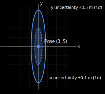
The inner dashed ellipse is the 1σ Mahalanobis contour; the outer solid ellipse is 2σ. They show greater uncertainty in y than in x. In 2D, the 1σ ellipse contains about 39.3% of the Gaussian probability mass (1 − e^{−1/2}), and the 2σ ellipse about 86.5% (1 − e^{−2}).
7. Summary
The entire Laplace approximation fits in three steps:
\[\begin{aligned} p(\mathbf x\mid\mathbf z) &\propto \exp[-L(\mathbf x)]\\[6pt] L(\mathbf x) &\approx L(\mathbf x^*)+ \frac12(\mathbf x-\mathbf x^*)^TH(\mathbf x-\mathbf x^*)\\[6pt] p(\mathbf x\mid\mathbf z) &\approx \mathcal N(\mathbf x^*,H^{-1}) \end{aligned}\]- Requirements: a sufficiently smooth loss, a local minimum (stationary point), and a positive-definite Hessian. It works best when the probability mass is concentrated around one dominant mode.
- Central insight: we are not claiming the original distribution is Gaussian. Near its maximum, its negative log-probability looks approximately quadratic, so the distribution looks locally Gaussian. That is the mathematical connection between optimization curvature and probabilistic uncertainty.
- Base assumption: the inverse Hessian is a statistically meaningful covariance only if the loss is a properly scaled negative log-posterior (or an appropriate likelihood-based approximation). For example, residuals must be weighted by their noise covariance, and the cost must not carry an extra factor: if a solver minimizes
Σ rᵀ Σ⁻¹ rwithout the½, its Hessian is2×the information matrix.