Metric 1 - Degeneracy using Hessian
Part 1 - The derivation
Suppose the state is
\[\mathbf{x} = \begin{bmatrix} \mathbf{p} \\ \mathbf{v} \\ \boldsymbol{\theta} \\ \mathbf{b}_a \\ \mathbf{b}_g \\ \mathbf{g} \end{bmatrix} \in \mathbb{R}^{18}.\]Each component is 3-dimensional, so the full state has 18 variables.
For each correspondence or measurement $i$, define a residual $\mathbf{r}_i(\mathbf{x})$. Its dimension $m$ depends on the registration method:
- Point-to-point ICP: $\mathbf{r}_i \in \mathbb{R}^3$
- Point-to-plane ICP: $r_i \in \mathbb{R}$
- Point-to-line ICP: often $r_i \in \mathbb{R}$, depending on the formulation
- NDT: can be represented with a 3D residual, $\mathbf{r}_i \in \mathbb{R}^3$, with the covariance used as a weighting or whitening term
For least-squares optimization, the cost of one measurement is (for simplicity we omit the information matrix $\Omega$)
\[E_i = \frac{1}{2}\mathbf{r}_i^T\mathbf{r}_i.\]The total cost is
\[E = \sum_i E_i = \frac{1}{2}\sum_i \mathbf{r}_i^T\mathbf{r}_i.\]Since $E_i$ is a scalar, its derivative with respect to the state is an $18\times1$ gradient.
Define the residual Jacobian as
\[\mathbf{J}_i = \frac{\partial \mathbf{r}_i}{\partial \mathbf{x}}.\]If the residual has dimension $m$, then
\[\mathbf{r}_i \in \mathbb{R}^{m}, \qquad \mathbf{J}_i \in \mathbb{R}^{m\times18}.\]- Point-to-plane ICP has $m=1$, so $\mathbf{J}_i \in \mathbb{R}^{1\times18}$.
- Point-to-point ICP has $m=3$, so $\mathbf{J}_i \in \mathbb{R}^{3\times18}$.
Using the chain rule,
\[\frac{\partial E_i}{\partial \mathbf{x}} = \mathbf{J}_i^T\mathbf{r}_i.\]After stacking all residuals into one vector,
\[\mathbf{r} = \begin{bmatrix} \mathbf{r}_0 \\ \mathbf{r}_1 \\ \vdots \end{bmatrix},\]and all residual Jacobians into one matrix,
\[\mathbf{J} = \begin{bmatrix} \mathbf{J}_0 \\ \mathbf{J}_1 \\ \vdots \end{bmatrix},\]the total cost becomes
\[E = \frac{1}{2}\mathbf{r}^T\mathbf{r},\]and its gradient is
\[\nabla E = \mathbf{J}^T\mathbf{r}.\]The Hessian is the derivative of the gradient:
\[\nabla^2 E = \frac{\partial^2 E}{\partial \mathbf{x}^2}.\]For a scalar residual $r_i$, the gradient of $E_i$ is
\[\nabla E_i = r_i \nabla r_i.\]Differentiating once more with the product rule gives
\[\nabla^2 E_i = (\nabla r_i)(\nabla r_i)^T + r_i\nabla^2 r_i.\]Since $\nabla r_i = \mathbf{J}_i^T$, we obtain
\[\nabla^2 E = \sum_i \left( \mathbf{J}_i^T\mathbf{J}_i + r_i\nabla^2 r_i \right).\]For a vector residual, the same idea applies component-wise:
\[\nabla^2 E = \mathbf{J}^T\mathbf{J} + \sum_k r_k \nabla^2 r_k.\]The first term, $\mathbf{J}^T\mathbf{J}$, depends only on the first derivatives of the residuals. The second term depends on their second derivatives and is weighted by the residual values themselves.
Near a good solution, the residuals $r_k$ are expected to be small. Gauss-Newton therefore neglects the second term and approximates the Hessian as
\[\boxed{\mathbf{H} \approx \mathbf{J}^T\mathbf{J}}\]For an 18-dimensional state,
\[\mathbf{J}^T\mathbf{J} \in \mathbb{R}^{18\times18}.\]This approximate Hessian describes how strongly the registration cost changes for different perturbations of the state.
Part 2 - Why Hessian eigenvalues can show degeneracy
Suppose we perturb the state $\mathbf{x}$ by a small amount $\delta\mathbf{x}$. A second-order Taylor expansion of the cost is
\[E(\mathbf{x}+\delta\mathbf{x}) \approx E(\mathbf{x}) + \nabla E(\mathbf{x})^T\delta\mathbf{x} + \frac{1}{2}\delta\mathbf{x}^T \mathbf{H}\, \delta\mathbf{x}.\]Near a local optimum,
\[\nabla E(\mathbf{x}) \approx 0,\]so the change in cost is approximately
\[E(\mathbf{x}+\delta\mathbf{x}) - E(\mathbf{x}) \approx \frac{1}{2}\delta\mathbf{x}^T \mathbf{H}\, \delta\mathbf{x}.\]Now consider the eigendecomposition of the Hessian:
\[\mathbf{H}\mathbf{v}_i = \lambda_i\mathbf{v}_i.\]Because the Hessian is symmetric, an $18\times18$ Hessian has 18 eigenvalues and we can choose 18 orthonormal eigenvectors,
\[\mathbf{v}_1,\ldots,\mathbf{v}_{18},\]which form a basis of the 18-dimensional error-state space.
Any state perturbation can therefore be written as
\[\delta\mathbf{x} = \sum_{i=1}^{18} a_i\mathbf{v}_i.\]Substituting this into the quadratic form gives
\[\delta\mathbf{x}^T \mathbf{H}\, \delta\mathbf{x} = \sum_{i=1}^{18} \lambda_i a_i^2.\]Therefore,
\[\boxed{ \Delta E \approx \frac{1}{2}\sum_{i=1}^{18} \lambda_i a_i^2 }\]Small eigenvalues
If an eigenvalue $\lambda_i$ is very small, then a perturbation along its eigenvector $\mathbf{v}_i$ changes the cost only slightly. For example, let
\[\delta\mathbf{x} = \alpha\mathbf{v}_i.\]Then
\[\Delta E \approx \frac{1}{2}\alpha^2\lambda_i.\]If
\[\lambda_i \approx 0,\]then
\[\Delta E \approx 0\]even for a nonzero perturbation $\alpha$. This means that changing the state along that direction produces almost no change in the registration cost. The measurements therefore provide little information about that state direction.
Here, a “direction” does not necessarily mean a physical direction in 3D space. The perturbation
\[\delta\mathbf{x}\in\mathbb{R}^{18}\]lives in the error-state space. An eigenvector might represent pure translation, pure rotation, or a combination of multiple state variables. For example, an eigenvector could look schematically like
\[\begin{bmatrix} 0.7 & 0.7 & 0 & 0 & \cdots & 0 \end{bmatrix}^T,\]meaning that the poorly observed direction is a combination of two state variables rather than a single coordinate axis.
Large eigenvalues
Conversely, suppose every eigenvalue is bounded away from zero:
\[\lambda_i \ge \lambda_{\min} > 0.\]Then
\[\sum_i \lambda_i a_i^2 \ge \lambda_{\min}\sum_i a_i^2.\]Because the eigenvectors are orthonormal,
\[\sum_i a_i^2 = \|\delta\mathbf{x}\|^2.\]Therefore,
\[\boxed{ \Delta E \gtrsim \frac{1}{2}\lambda_{\min}\|\delta\mathbf{x}\|^2 }\]So if the smallest eigenvalue is sufficiently far from zero, there is no nonzero unit state direction that can be changed without noticeably increasing the cost. In that sense, there is no locally unobservable direction in the Hessian.
“Small” or “large” eigenvalues are relative quantities. In an 18-state LIO system, different state components have different units, such as meters, radians, meters per second, and sensor-bias units. For this reason, LiDAR geometric degeneracy is often analyzed using the $6\times6$ pose Hessian associated with translation and rotation rather than the full $18\times18$ estimator Hessian.
Plane is a Natural Degeneracy Scenario
Some point-cloud geometries naturally provide weak constraints on certain pose directions. A common example is a single plane.
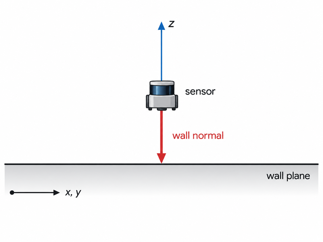
Imagine the robot facing a large flat wall. In point-to-plane ICP, each residual measures displacement along the wall normal. If the robot moves parallel to the wall, the point-to-plane residuals change very little. Therefore,
\[\mathbf{J}\delta\mathbf{x} \approx 0,\]and consequently
\[\Delta E \approx \frac{1}{2} \delta\mathbf{x}^T \mathbf{H} \delta\mathbf{x} \approx 0.\]These weakly constrained motions appear as small eigenvalues of the pose Hessian.
For an ideal infinite plane, two translations along the plane are unobservable. Rotation about the plane normal is also unobservable in pure point-to-plane ICP. Therefore, an ideal single-plane geometry can produce three near-zero eigenvalues in the $6\times6$ pose Hessian.
Other common degeneracy cases include long corridors or tunnels, line-like structures, scenes dominated by parallel planes, narrow fields of view, and highly repetitive or symmetric geometry. In each case, the underlying issue is the same: some pose perturbation changes the measured geometric residuals very little.