This post builds on the pipeline in LIO Hands-On.
Baseline: PCL NDT LIO
Using stock PCL 1.14 NDT, our LIO pipeline averaged 26.6 ms per frame, including 24.0 ms for scan matching and 1.9 ms for preprocessing. Profiling showed these bottlenecks (share of CPU samples):
| Hotspot | CPU samples |
|---|---|
| NDT derivative computation | ~32% |
| FLANN k-d tree operations | ~16% |
| Radius outlier removal | ~10% |
| Memory allocation | ~8% |
- PCL computes NDT derivatives in a single thread, limiting parallelism.
pcl::Registration::align()rebuilds a k-d tree over the entire target after each map update, even though NDT itself does not use it for alignment. The only consumer isgetFitnessScore(), which searches the raw target points.- Rebuilding the ~246k-point local map (see Local Map Rebuild) took 7.2 ms per keyframe on a background thread. Since the next
align()waits on that future, this occasionally added 1.5 ms of waiting time to scan matching.
Improving LIO Accuracy: What Worked
Our main challenges were drift along featureless corridors and poor scan matching during fast rotations. We tested several approaches to improve accuracy, and three changes produced the most significant improvements.
1. Coarse-to-Fine NDT Matching
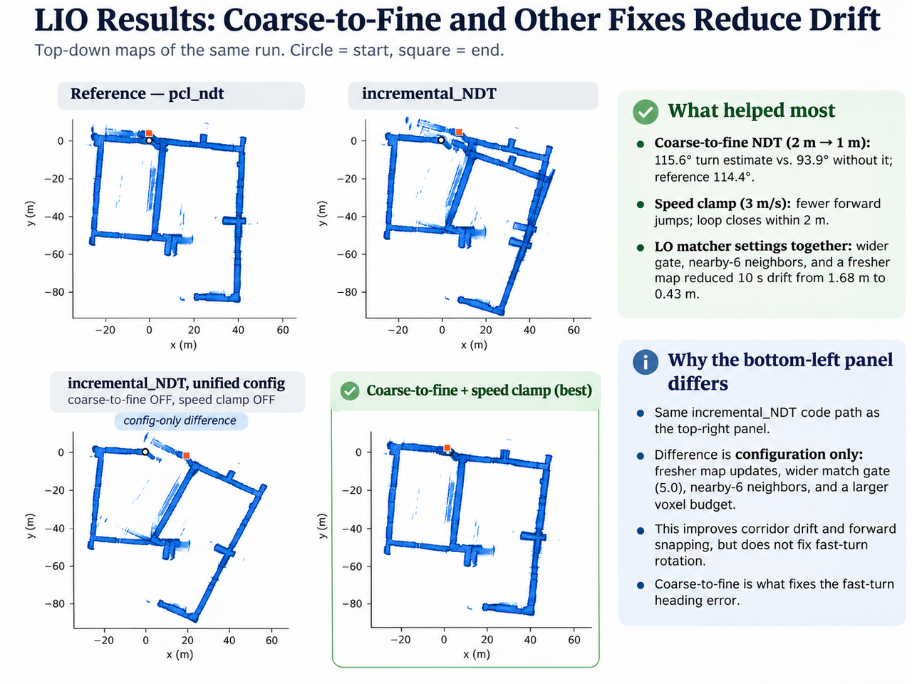
We introduced a two-stage alignment process: first matching against a coarse 2 m voxel map, then refining against a 1 m map. During a fast rotation at 12.5–15 s, this improved the estimated turn from 93.9° to 115.6°, compared with the reference of 114.4°.
The underlying problem was the inaccurate IMU prediction, which captured only 78° of a 153° turn. At 1 m resolution, the initial misalignment was too large for reliable voxel correspondences, limiting corrections to roughly 5–10° per frame. The coarse map provided a larger convergence basin, allowing the fine matcher to refine a much better initial estimate.
2. Limiting Matched Velocity To 3 m/s
Long, featureless corridors provide weak constraints on translation along their length. As a result, scan matching occasionally produced large forward jumps. Since the robot typically travels at around 1 m/s, we introduced a 3 m/s limit on matched motion. This reduced unrealistic jumps and helped achieve loop closure within 2 m.
3. Combining Wider Matching Gates, Neighboring Voxels, And Frequent Map Updates (LO)
In lidar-only odometry (LO), we combined:
- A wider matching gate: point-voxel pairs are rejected when their squared Mahalanobis distance exceeds 5.0.
- A search over the six face-adjacent voxels as well as the point’s own voxel (see Multi-Neighbor NDT).
- Map updates every second scan.
Together, these reduced 10-second drift from 1.68 m to 0.43 m.
These improvements worked together: the wider gate retained points with larger initial alignment errors, neighboring voxels improved matching near cell boundaries, and more frequent map updates reduced empty cells near the robot. Individually, these changes provided little improvement or sometimes degraded performance.
What Didn’t Work: Seven Failed Experiments
Not every modification improved LIO accuracy. Several experiments exposed underlying limitations in scan matching, inertial propagation, and map consistency. The failures fall into four categories.
1. Geometric Constraints That Reinforced Existing Errors
A. Constraining motion along the floor normal (LO)
We fitted a floor plane to each scan and removed translation along its normal:
1
2
3
n = fit_floor_normal(scan)
dz = dot(pose.t - prev.t, n)
pose.t -= dz * n
Result: Tilt diverged to 114°, while position jumps exceeding 0.3 m increased from 20 to 48.
Explanation: The floor normal was estimated using the current pose. Once the pose tilted, the estimated normal tilted with it, potentially introducing corrections along the wrong direction. The scan matcher then compensated through rotation, reinforcing the error.
The key limitation was that the floor constraint was not independent of the pose estimate. A more reliable constraint would use an external reference, such as gravity estimated from accelerometer measurements.
B. Hessian-based degeneracy handling
We attempted to suppress pose updates along weakly observable directions using the eigenvalues of the 6×6 Gauss–Newton Hessian:
1
2
3
lam, V = eig(H)
weak = lam < threshold * lam.max()
dx = V @ diag(~weak) @ V.T @ solve(H, b)
Result: The method never activated at relative thresholds of 1e-3 or 1e-2. Increasing the threshold to 5e-2 caused the estimated path to shrink to 220 m and tilt to reach 41°.
Explanation: The weakest Hessian eigenvalue was approximately 3% of the strongest, so it stayed above the 1e-3 and 1e-2 thresholds. Although corridor geometry provided relatively weak constraints in certain directions, those directions were not completely unobservable.
The dominant issue appeared to be biased correspondences rather than missing information. Eigenvalue thresholding measures local sensitivity, but cannot determine whether otherwise informative correspondences are systematically wrong. Increasing the threshold simply discarded useful information.
2. Optimization Changes That Reduced Robustness
C. Magnusson score instead of gated Mahalanobis error
We replaced the gated Mahalanobis objective with Magnusson’s bounded exponential score:
1
2
3
4
5
6
7
8
# r = e.T @ inv(Sigma) @ e

# Original: minimized
cost = sum(r for r in residuals if r <= 5)

# Magnusson: maximized (d1 < 0, so each term is positive)
score = sum(-d1 * exp(-0.5 * d2 * r)
            for r in residuals)
Result: The LO trajectory produced its best loop shape, but its height varied by up to +4.9 m. LIO performed worse, with a worst leg ratio of 0.32.
Likely explanation: The exponential weighting strongly suppresses large residuals. This may have reduced the influence of relatively sparse floor and ceiling correspondences, weakening vertical constraints while preserving horizontal alignment from the more numerous wall points.
In LIO, inaccurate IMU predictions also produced larger initial misalignments, potentially pushing more correspondences into the low-weight region.
This objective improved some aspects of horizontal geometry but introduced unacceptable vertical drift.
D. Smoothed-velocity initialization (LO)
We used an exponentially smoothed velocity estimate to initialize each scan match:
1
2
v = alpha * v + (1 - alpha) * delta_position / dt
init_guess.t = prev_pose.t + v * dt
Result: Estimated path length varied between 284 m and 339 m depending on the smoothing factor, compared with approximately 332 m for the reference.
Explanation: Translation along a featureless corridor is weakly constrained. Consequently, the matcher often converged near its starting guess rather than correcting the initial translation error.
Changing the velocity smoothing factor changed the estimated trajectory without resolving the underlying ambiguity.
3. Over-Reliance On Unreliable IMU Predictions
E. Increasing ESKF pose measurement noise
We increased the scan-matching pose measurement noise from 1e-3 to values including 0.05 and 0.2, reducing the influence of scan-matching updates.
Result: The filter diverged, even when using PCL NDT.
Explanation: The dataset contained IMU measurements at approximately 27 Hz instead of the expected 100 Hz, with roughly 88% of samples missing and some intervals exceeding 0.1 s.
Increasing measurement noise shifted more responsibility to inertial propagation, which was unreliable under these sampling conditions. The filter required strong corrections from scan matching to remain stable.
F. Rejecting unsuccessful scan matches
We tested rejecting scans when the matcher failed to converge or produced anomalous scores:
1
2
3
4
ok = matcher.align(guess)

if not ok or anomaly(score):
    skip_update()  # Keep IMU prediction
Result: PCL NDT rejected 5,044 of 5,204 frames, causing the trajectory to diverge.
Explanation: Under the tested configuration, PCL frequently reached its iteration limit without reporting convergence, even when the estimated alignment remained useful.
Using its convergence flag as a strict acceptance criterion effectively disabled most scan-matching corrections, leaving the sparse IMU measurements to determine the trajectory.
A more effective alternative was a 3 m/s physical speed limit, which rejected implausible translational jumps without relying solely on the optimizer’s convergence status.
4. Excessively Frequent Map Updates
G. Updating the map every scan
We increased the map insertion frequency from every second scan to every scan:
1
2
3
4
keyframe_frame_gap = 1

if is_keyframe(k):
    map.add(scan_world)
Result: There was no measurable improvement without coarse-to-fine alignment. With coarse-to-fine enabled, the worst leg ratio worsened to 2.39.
Possible explanation (low confidence): Each scan is inserted using its estimated pose. Small alignment errors can therefore enter the map, influence subsequent matching, and then compound.
Updating every second scan may reduce this effect by retaining the previous map for another matching step. The coarse 2 m voxel map could be particularly sensitive because errors in inserted points can shift voxel statistics and influence the initialization of the fine alignment.
This interpretation remains a hypothesis; additional experiments would be needed to isolate the effect of update frequency.