Magnusson NDT
The NDT in 3D SLAM - 1 is a plain least-squares problem: each point’s cost grows without bound as it moves away from its voxel mean. The problem of this approach is that a badly matched point-voxel pair could contribute significantly to the final loss and gradients. Magnusson’s NDT, which PCL’s pcl::NormalDistributionsTransform implements, instead scores each point with a Gaussian such that for the badly matched point-voxel pair:
- The penalty approaches a constant instead of growing forever.
- The gradient contribution decays exponentially toward zero instead of growing linearly with the residual.
1. The Design: The Penalty Saturates Instead Of Growing Indefinitely
For a source point p transformed by the pose T, the residual to its voxel mean μ and its squared Mahalanobis distance are:
where Ω is the voxel’s information matrix.
Vanilla least squares:
\[\begin{gather*} E_{\mathrm{LS}}=\frac12 r \longrightarrow\infty \end{gather*}\]Magnusson’s per-point score is:
\[\begin{gather*} s = -d_1 \exp\left(-\frac{d_2}{2} r\right) = -d_1 \exp\left(-\frac{d_2}{2} (Tp - \mu)^T \Omega (Tp - \mu)\right) \end{gather*}\]where d_1 and d_2 are constants fitted so that a Gaussian plus a uniform outlier floor is approximated by a single Gaussian. Up to scale and offset, it’s equivalent to this normalized penalty:
With PCL’s parameterization, d_1 < 0 and d_2 > 0, so s is positive and peaks at r = 0. PCL maximizes s, which is the same as minimizing E_M.
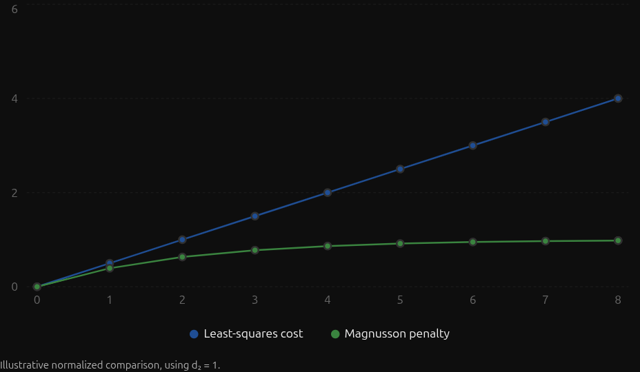
- Vanilla: The penalty keeps growing as the point gets farther from the voxel.
- Magnusson: The penalty saturates. Once a point is sufficiently far away, moving it even farther has little effect.
2. The Gradient Approaches Zero
With J = ∂e/∂θ the Jacobian of e with respect to the pose θ (derivation in Appendix 1):
Vanilla:
\[\begin{gather*} g_{\mathrm{LS}}=J^T\Omega e \end{gather*}\]This gradient grows linearly with the residual magnitude ||e||, not with r, because r is already a squared distance.
Magnusson:
\[\begin{gather*} g_{\mathrm{M}}=d_2\underbrace{\exp(-d_2r/2)}_{\text{exponential downweighting}} J^T\Omega e \end{gather*}\]As r → ∞, the exponential decays faster than ||e|| grows, so:
Why Is That Useful?
Imagine a LiDAR scan with 1,000 points:
- 950 points match the map well.
- 50 points belong to an object that isn’t in the map.
With vanilla least squares, those 50 badly matched points can pull the pose estimate strongly. With Magnusson, they contribute almost nothing once their residuals are large.
Magnusson isn’t more stable because its penalty is smaller. It’s more robust to outliers because badly matched points have bounded influence on the optimization.
Weakness: It Needs A Good Initial Guess
When the initial transform is far off, many correct points also have large residuals, so they get downweighted just like outliers. The useful gradient then disappears and the optimizer can stall or converge to the wrong pose. For a real example, see experiment C in LIO Accuracy, where Magnusson’s score caused up to 4.9 m of vertical drift.
Appendices
Appendix 1 - Deriving Magnusson’s Gradient
Define:
\[\begin{gather*} r=e^T\Omega e,\qquad w=\exp(-d_2r/2) \end{gather*}\]First, differentiate the squared Mahalanobis distance:
\[\begin{gather*} \frac{\partial r}{\partial\theta} =2J^T\Omega e \end{gather*}\]Now apply the chain rule to s = -d_1 w:
Substituting:
\[\begin{gather*} \boxed{ g_{\mathrm{NDT}}=d_1d_2wJ^T\Omega e } \end{gather*}\]Compare this with ordinary least squares:
\[\begin{gather*} g_{\mathrm{LS}}=J^T\Omega e \end{gather*}\]Same Jacobian, but the Magnusson gradient is scaled by d_1 d_2 w. Because w decays exponentially as the residual grows, distant points contribute much less to the gradient. Since d_1 < 0, g_NDT = -|d_1| g_M: ascending s is the same as descending E_M from section 2.
Appendix 2 - Magnusson’s Full Hessian
This is where the biggest mathematical difference appears.
Let:
\[\begin{gather*} a=J^T\Omega e \end{gather*}\]And define the second derivative of the transformed point:
\[\begin{gather*} K_{ij}=\frac{\partial^2e}{\partial\theta_i\partial\theta_j} \in\mathbb R^3 \end{gather*}\]Write the gradient component by component, then differentiate it again:
\[\begin{gather*} g_i=d_1d_2w\,a_i \end{gather*}\]Using the product rule:
\[\begin{gather*} \frac{\partial g_i}{\partial\theta_j} =d_1d_2\left( \frac{\partial w}{\partial\theta_j}a_i+ w\frac{\partial a_i}{\partial\theta_j} \right) \end{gather*}\]The two terms are:
\[\begin{gather*} \frac{\partial w}{\partial\theta_j} =-d_2wa_j \end{gather*}\] \[\begin{gather*} \frac{\partial a_i}{\partial\theta_j} =J_i^T\Omega J_j+e^T\Omega K_{ij} \end{gather*}\]Therefore:
\[\begin{gather*} \boxed{ H_{\mathrm{NDT},ij} =d_1d_2w \left[ J_i^T\Omega J_j +e^T\Omega K_{ij} -d_2a_ia_j \right] } \end{gather*}\]Or, in matrix form:
\[\begin{gather*} \boxed{ H_{\mathrm{NDT}} =d_1d_2w \left[ J^T\Omega J+B-d_2aa^T \right] } \end{gather*}\]where B_ij = e^T Ω K_ij.
Unlike the Gauss-Newton approximation J^T Ω J, which is always positive semi-definite, this Hessian has the B and -d_2 a a^T terms, so it can be indefinite for points far from their voxel mean. That’s why the optimizer needs a line search (PCL uses Moré-Thuente) instead of trusting the full Newton step.