Nodes Are Pose Corrections, Not Poses
In traditional SLAM, a node contains an unknown robot pose:
\[\begin{gather*} x_k=(x,y,\theta) \end{gather*}\]The INS already provides poses, so this graph doesn’t optimize them directly. Instead:
\[\begin{gather*} \boxed{x_k^{\text{corrected}}=x_k^{\text{INS}}+d_k} \end{gather*}\]where d_k is the unknown east/north correction at time k. In this implementation, a node in the graph is the unknown pose correction.
| Time | INS east | Graph variable d_k |
Corrected east |
|---|---|---|---|
| 10 s | 100.0 m | +0.2 m | 100.2 m |
| 12 s | 102.0 m | +0.3 m | 102.3 m |
| 14 s | 104.0 m | +0.1 m | 104.1 m |
Modeling The Correction As A Gauss-Markov Process
At 10 seconds, perhaps the correction needed is +30 cm. At 12 seconds, it’s probably still somewhere near +30 cm. At 14 seconds, it could be +25 cm. At 30 seconds, it might be quite different.
Gauss-Markov is a mathematical way of saying that errors close together in time tend to be similar, but the relationship weakens as time passes. So this is a probabilistic view of the INS error:
\[\begin{gather*} \boxed{d_{k+1}=\phi d_k+w_k} \end{gather*}\]d_k: correction needed at the current time.d_{k+1}: correction needed at the next time.φ: how much of the previous correction tends to persist.w_k: an unpredictable random change, modeled as Gaussian noise with varianceQ.
For example, with nodes 2 s apart and a correlation time of 30 s, suppose the correction at 10 s is exactly 0.30 m:
\[\begin{gather*} d_{10}=0.30\text{ m}, \qquad \phi=e^{-2/30}\approx0.936 \\ d_{12}=0.936(0.30)+w \\ \boxed{d_{12}=0.281+w} \end{gather*}\]E.g., if w = 0.04 m, the next correction is 0.321 m. Since φ < 1, the expected correction slowly decays toward zero.
Some other similar probabilistic models are:
- Random walk:
d_{k+1} = d_k + w_k. - Constant correction:
d_{k+1} = d_k.
Fitting It Into Graph Optimization
Let the residual of an edge connecting two neighboring correction nodes be:
\[\begin{gather*} \boxed{r_k=d_{k+1}-\phi d_k} \\ E_k=\frac{(d_{k+1}-\phi d_k)^2}{Q} \end{gather*}\]where Q is the assumed variance of the process disturbance. These edges link neighboring INS correction nodes. If we move one node away from what its neighbor predicts, we get more penalty, like more tension in a spring.
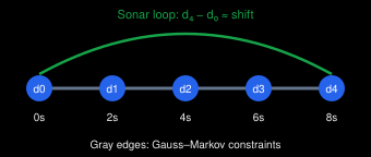
Example: One Sonar Loop Closure
Initially, all corrections are zero:
\[\begin{gather*} d_0=d_1=d_2=d_3=d_4=(0,0) \end{gather*}\]Suppose the texture matcher finds that the correction difference between node 0 and node 4 should be:
\[\begin{gather*} \boxed{s = d_4-d_0\approx(0.3,-0.1)\text{ m}} \end{gather*}\]Then the solver minimizes:
\[\begin{gather*} E= \underbrace{\frac{d_0^2}{\sigma^2}}_{\text{initial prior}} + \underbrace{\sum_{k=0}^{3}\frac{(d_{k+1}-\phi d_k)^2}{Q}}_{\text{Gauss-Markov edges}} + \underbrace{\frac{(d_4-d_0-s)^2}{\sigma_L^2}}_{\text{sonar loop}} \end{gather*}\]With φ = 0.936, σ = 0.5 m, Q = (1 - φ²)σ² ≈ 0.031 m² (see the next section), and σ_L = 0.05 m, the solution is:
| Node | East correction (m) | North correction (m) |
|---|---|---|
d_0 |
−0.15 | +0.05 |
d_1 |
−0.07 | +0.02 |
d_2 |
0.00 | 0.00 |
d_3 |
+0.07 | −0.02 |
d_4 |
+0.15 | −0.05 |
The loop’s correction is spread evenly along the chain. d_4 - d_0 is slightly less than s because the loop closure has its own uncertainty σ_L.
Keeping The Variance From Growing Forever
One detail is we want the INS correction to fluctuate over time, but we don’t want its uncertainty to grow forever (which is what a random walk does). For
\[\begin{gather*} d_{k+1}=\phi d_k+w_k \end{gather*}\]w_k: new independent Gaussian noise, with varianceQ.σ²: the desired long-term variance ofd_k,d_{k+1}, …
After multiplying by φ, the variance of φ d_k is φ²σ². Variances of independent variables add, and we want d_{k+1} to have variance σ² too:
For example, with φ = 0.8 and σ = 1 m, we want the correction’s variance to remain at 1 m² over time, so Q = 1 - 0.64 = 0.36 m².
Solving The Graph
All constraints contribute to a least-squares objective:
\[\begin{gather*} \boxed{E(d)=\frac12d^\top H d-b^\top d+C} \end{gather*}\]where:
d: all the unknown node corrections.H: the information matrix, calledinformationin the code.b: the information vector, calledinformation_vectorin the code.C: a constant that doesn’t affect the optimization.
We minimize this objective by setting its derivative to zero:
\[\begin{gather*} \frac{\partial E}{\partial d}=Hd-b=0 \\ \boxed{Hd=b} \quad \Rightarrow \quad \boxed{d^*=H^{-1}b} \end{gather*}\]Step A: Build The Information Matrix
1
information = np.zeros((n, n))
At this point, the graph has no constraints. The Gauss-Markov prior adds terms to information:
1
2
3
4
information[k + 1, k + 1] += 1.0 / step_variance
information[k, k] += phi**2 / step_variance
information[k, k + 1] -= phi / step_variance
information[k + 1, k] -= phi / step_variance
This creates the mathematical connection between adjacent correction nodes. These four lines are aaᵀ / Q for the residual r_k = d_{k+1} - φ d_k, whose row a has -φ at index k and 1 at index k + 1. Here step_variance is Q.
Step B: Add Loop Closures
For a sonar loop with measured displacement s, the residual is:
Here, a is a vector that selects the two timestamps’ corrections (+1 at one, -1 at the other), using interpolation weights between neighboring nodes if needed. The loop contributes:
1
2
3
4
5
information += np.outer(row, row) / model.loop_std_m**2
information_vector += (
    np.outer(row, (shift_east, shift_north))
    / model.loop_std_m**2
)
Mathematically:
\[\begin{gather*} H\leftarrow H+\frac{aa^\top}{\sigma_L^2} \\ b\leftarrow b+\frac{as}{\sigma_L^2} \end{gather*}\]The first update modifies the system’s coefficients. The second adds the measured shift. East and north share the same H, so b has two columns, one per axis.
Step C: Solve
1
2
covariance = np.linalg.inv(information)
offsets_m = covariance @ information_vector
The code computes:
\[\begin{gather*} \Sigma=H^{-1} \\ \boxed{d^*=\Sigma b} \end{gather*}\]Σ is also the covariance of the optimized corrections, which is why the code computes the full inverse instead of only solving Hd = b. offsets_m is the optimized result, and every row contains the optimized correction at one timestamp:
1
2
3
4
5
6
7
offsets_m =
[
    [d0_east, d0_north],
    [d1_east, d1_north],
    [d2_east, d2_north],
    ...
]
H must be invertible. The Gauss-Markov edges and loop closures mostly constrain differences between corrections, so the prior on d_0 is what keeps H well-conditioned.
Concrete Example With Two Nodes
Let’s simplify the problem to one dimension:
- Two unknown corrections:
d_0,d_1. - A prior prefers both corrections near zero.
- A sonar loop says
d_1 - d_0 ≈ 0.3m. - For illustration, all three residuals have equal weight.
The objective is:
\[\begin{gather*} E=d_0^2+d_1^2+(d_1-d_0-0.3)^2 \end{gather*}\]Taking derivatives and dividing by 2 gives:
\[\begin{gather*} \underbrace{\begin{bmatrix} 2&-1\\ -1&2 \end{bmatrix}}_{H} \underbrace{\begin{bmatrix}d_0\\d_1\end{bmatrix}}_{d} = \underbrace{\begin{bmatrix}-0.3\\0.3\end{bmatrix}}_{b} \end{gather*}\]Solve:
\[\begin{gather*} \boxed{d_0=-0.1,\qquad d_1=+0.1} \end{gather*}\]The graph distributes the correction between the two nodes. The loop residual is:
\[\begin{gather*} d_1-d_0-0.3=0.1+0.1-0.3=-0.1\text{ m} \end{gather*}\]The loop isn’t fully satisfied, because the priors pull both corrections toward zero with the same weight as the loop.
Linear Vs. Nonlinear Graphs
This Graph Is Linear
The node is:
\[\begin{gather*} d_i=[\Delta x_i,\Delta y_i] \end{gather*}\]The loop residual is:
\[\begin{gather*} \boxed{r_{ij}=d_j-d_i-s_{ij}} \end{gather*}\]where s_ij is the measured sonar shift. The Gauss-Markov residual is:
Both are linear in d, so their Jacobians are constant. Therefore, we can solve Hd = b once, without Gauss-Newton iterations. This is the same reason plane fitting doesn’t need Gauss-Newton.
What If We Also Optimize Yaw?
Suppose the node becomes a full 2D pose:
\[\begin{gather*} x_i=[p_{x,i},p_{y,i},\theta_i] \end{gather*}\]For conventional relative-pose constraints, the translation residual becomes:
\[\begin{gather*} \boxed{r_{ij}^{t}=R(\theta_i)^\top(p_j-p_i)-z_{ij}^{t}} \\ R(\theta_i)= \begin{bmatrix} \cos\theta_i&-\sin\theta_i\\ \sin\theta_i&\cos\theta_i \end{bmatrix} \end{gather*}\]Now the residual contains sin θ_i, cos θ_i, and their products with the unknown positions. That’s nonlinear: the Jacobian depends on the current estimate, so we have to linearize around it, solve, update, and repeat with Gauss-Newton or Levenberg-Marquardt.