Consider gradient descent:
\[\theta_{t+1}=\theta_t-\eta_t\nabla L(\theta_t)\]Where:
θ_t: model parameters at steptη_t: learning rate at stept∇L: gradient of the loss
Warmup
Warmup: the learning rate starts small and increases linearly. Suppose our target learning rate is 0.001 and warmup lasts 10 epochs:
| Epoch | Without warmup | With warmup |
|---|---|---|
| 1 | 0.001 | 0.0001 |
| 2 | 0.001 | 0.0002 |
| 5 | 0.001 | 0.0005 |
| 10 | 0.001 | 0.001 |
A typical schedule starts at a small learning rate, gradually increases it to the target value, then decreases it. Starting with a large learning rate makes training more likely to go unstable: the weights are random, so early gradients can be large and the updates can overshoot. For Adam, the moving estimates of the gradient moments are also built from only a few batches at first, so they are noisy and the adaptive step size is unreliable.
LambdaLR
PyTorch’s LambdaLR uses:
1
learning_rate = base_learning_rate * lr_lambda(step)
For example,
1
2
3
4
5
6
7
8
9
import math

def lr_lambda(epoch):
    return 0.5 * (1 + math.cos(math.pi * epoch / 100))

# at epoch 0,   lr_lambda = 1    (full base learning rate)
# at epoch 50,  lr_lambda = 0.5
# at epoch 100, lr_lambda = 0
scheduler = torch.optim.lr_scheduler.LambdaLR(optimizer, lr_lambda)
One implementation detail: the argument of lr_lambda is just how many times scheduler.step() has been called. So whether it means “epoch” or “batch” depends on where you call scheduler.step(): once per epoch, or once per optimizer update. E.g., per batch:
1
2
3
4
5
6
7
for epoch in range(total_epochs):
    for batch in loader:
        optimizer.zero_grad()
        loss = compute_loss(model, batch)
        loss.backward()
        optimizer.step()
        scheduler.step()   # after optimizer.step()
When stepping per batch, write lr_lambda in terms of total steps (total_epochs * len(loader)), not epochs.
Warmup + Cosine Decay
Example: warmup over epochs 0–10, then cosine decay over epochs 10–100. With decay progress
\[p=\frac{\text{epoch}-10}{100-10}\in[0,1], \qquad \text{LR multiplier}=\frac{1+\cos(\pi p)}{2}\]Because the normalized progress p ranges from 0 to 1, the angle πp ranges only from 0 to π: half a cosine period, where the cosine falls from 1 to −1.
| Decay progress | Cosine value | LR multiplier |
|---|---|---|
| 0% | 1 | 1 |
| 25% | 0.707 | 0.854 |
| 50% | 0 | 0.5 |
| 75% | −0.707 | 0.146 |
| 100% | −1 | 0 |
The learning rate decreases monotonically, never increasing during this phase. Both phases fit in one LambdaLR:
1
2
3
4
5
def lr_lambda(epoch):
    if epoch < 10:
        return (epoch + 1) / 10                    # warmup: 0.1, 0.2, ..., 1.0
    p = (epoch - 10) / 90
    return 0.5 * (1 + math.cos(math.pi * p))       # cosine decay: 1 -> 0
There are other schedules, like cosine annealing with warm restarts, where the learning rate periodically rises again, but ordinary warmup + cosine decay doesn’t do that within its configured interval.
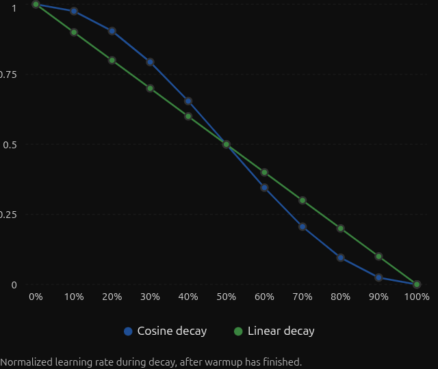
(In this example, the schedule changes once per epoch. You can also advance it once per training batch.)
Cosine Annealing
In metallurgy, annealing means heating a material and then cooling it slowly so its structure settles into a stable, low-energy state. In machine learning, cosine annealing is a learning rate schedule that starts high and is gradually lowered along a cosine curve:
\[\eta(t)=\eta_{\min}+\frac{1}{2}\left(\eta_{\max}-\eta_{\min}\right)\left(1+\cos\left(\frac{\pi t}{T}\right)\right)\]Where:
η(t): learning rate at steptη_max: maximum learning rateη_min: minimum learning rateT: total decay steps
Does cosine annealing use the first half of the cosine curve? Yes. t/T goes from 0 to 1, so the angle πt/T goes from 0 to π. That is the falling half of the cosine: η(0) = η_max, η(T/2) is the midpoint, and η(T) = η_min. It is the same formula as the cosine decay above, with η_min = 0 there.
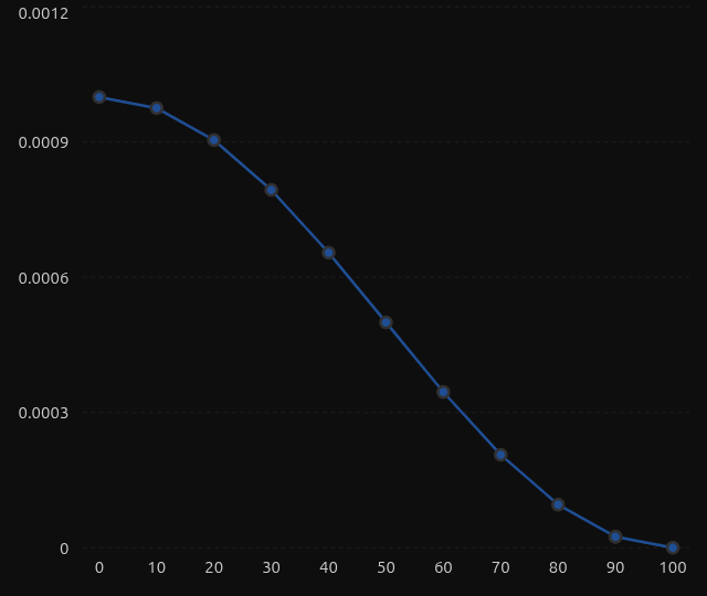
Another algorithm is SGDR (Stochastic Gradient Descent with Warm Restarts, Loshchilov & Hutter, 2017). Instead of decaying the learning rate only once, it periodically jumps it back to η_max and decays again:
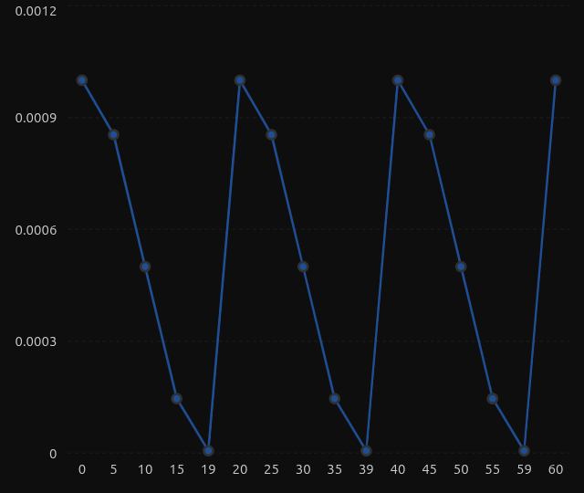
The jump encourages the optimizer to move away from its current region and explore other solutions.
PyTorch implements these approaches separately:
1
2
3
4
5
6
7
8
9
10
11
12
13
# Cosine decay from the base LR to eta_min over T_max scheduler steps
torch.optim.lr_scheduler.CosineAnnealingLR(
    optimizer,
    T_max=100,
    eta_min=0
)

# Cosine decay with periodic warm restarts
torch.optim.lr_scheduler.CosineAnnealingWarmRestarts(
    optimizer,
    T_0=20,     # steps in the first cycle
    T_mult=1    # each later cycle is T_mult times longer (1 = all cycles equal)
)
Neither includes warmup. Use LambdaLR as above, or chain LinearLR and CosineAnnealingLR with SequentialLR. Also, if CosineAnnealingLR is stepped past T_max, the learning rate follows the cosine back up instead of staying at eta_min, so set T_max to the real number of steps.