Supervised contrastive learning (SupCon) trains a model to produce embeddings in which images of the same class are close together and images of different classes are far apart. Ordinary classification only asks the model to predict the correct label; SupCon also explicitly trains the relationships between feature vectors.
1. The Basic Idea
Imagine a dataset of cats and dogs:
| Cat — Image A | Cat — Image B | Dog — Image C | Dog — Image D |
|---|---|---|---|
 |
 |
 |
 |
- An ordinary classifier learns to answer: is this image a cat or a dog?
- SupCon adds another objective: make the embeddings of different cats similar to one another, and distinguish them from dog embeddings. For example, the two cats should have similar embeddings even though their colors and appearances differ.
2. Training Architecture
A typical image classifier:
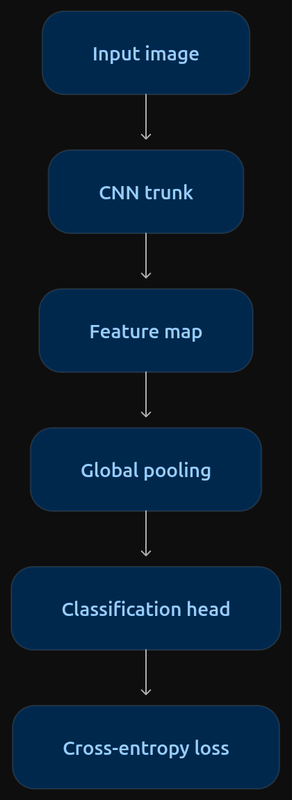
SupCon adds a separate projection head and a contrastive loss:
.png)
Both branches share the CNN trunk. During training, cross-entropy teaches the network to classify images, while SupCon encourages the embeddings to have meaningful class-based relationships. The projection head is typically a small MLP, and its output is L2-normalized before computing similarities. The projection head can be discarded after training.
3. Measuring Similarity
Each image is passed through the CNN and projection head to produce an embedding vector. For two embeddings z_i and z_j, the cosine similarity is below; if both embeddings are already L2-normalized, it simplifies to a dot product:
Cosine similarity ranges from -1 to 1, where 1 means the vectors point in the same direction. Suppose we obtain the following similarities:
| Pair | Similarity | Desired behavior |
|---|---|---|
| A–B (cat–cat) | 0.30 | Increase |
| A–C (cat–dog) | 0.80 | Decrease |
| A–D (cat–dog) | 0.10 | Already relatively low |
The problem is that Image A (cat) is more similar to Image C (dog) than to Image B (cat). Contrastive loss penalizes this arrangement.
4. Supervised Contrastive Loss
One commonly used supervised contrastive loss is:
\[\boxed{ \mathcal L_i = -\frac{1}{|P(i)|} \sum_{p\in P(i)} \log \frac{\exp(s_{ip}/\tau)} {\sum_{a\ne i}\exp(s_{ia}/\tau)} }\]where:
i: the anchor image, i.e. the image currently being compared against the others.P(i): the set of positives, the other images in the batch with the same class label asi.|P(i)|is how many there are, so the loss averages over all positives. Each term is the softmax probability of one positive, so the more similar same-class images are, the lower the loss.s_ip: cosine similarity between the anchor and a positive image.τ: temperature, controlling how strongly similarity differences affect the loss.a: any other image in the batch, positive or negative.
For our example, Image A is the anchor, Image B is the only positive, and C and D are negatives. With τ = 0.1, the softmax probability assigned to B, and the resulting loss, are:
5. Combining Classification and Contrastive Losses
The ordinary classification loss is still present:
\[\boxed{ \mathcal L_{\text{total}} = \mathcal L_{\text{CE}} + \lambda\mathcal L_{\text{SupCon}} }\]where:
L_CE: cross-entropy loss for predicting cat versus dog.L_SupCon: contrastive loss that organizes embeddings by class.λ: hyperparameter controlling the relative importance of contrastive learning.
The original SupCon paper (Khosla et al., 2020) trains in two stages instead: first the encoder with SupCon alone, then a linear classifier on top of the frozen encoder. Adding the two losses together as above is a common single-stage variant.
6. Summary
- In ordinary supervised classification, we train the model to predict the correct class.
- In supervised contrastive learning, we additionally train the model to organize its embedding space by class.
- The network isn’t explicitly told where to place each embedding. It learns feature representations through gradient descent on the contrastive loss.
- For cat and dog classification, this means images of different cats produce relatively similar embeddings, while cat and dog embeddings become easier to distinguish.