How a Decoder-Only LLM Is Trained
Suppose we want to train a model to answer questions. Consider this training example:
1
[BOS] [USER] What do you see ? [ASSISTANT] I see a robot
Here, [BOS] is a beginning-of-sequence token, while [USER] and [ASSISTANT] indicate the roles in the conversation.
Conceptually, autoregressive language-model training asks the same question repeatedly:
Given all the tokens I have seen so far, what should the next token be?
For the assistant response, we can think of training as the following sequence of prediction problems.
Conceptual sequential view
Step 1
1
2
3
4
5
6
7
8
Input:
[BOS] [USER] What do you see ? [ASSISTANT]

Model prediction:
"You"

Correct next token:
"I"
The model may be wrong and assign a high probability to "You", but the loss is calculated using the correct token:
For the next conceptual step, we use the ground-truth token "I", not the model’s incorrect prediction "You". This is called teacher forcing; see Series 5 for how it can cause exposure bias.
Step 2
1
2
3
4
5
6
7
8
Input:
[BOS] [USER] What do you see ? [ASSISTANT] I

Model prediction:
"are"

Correct next token:
"see"
The loss is
\[L_2 = -\log P( \text{"see"} \mid \text{[BOS] [USER] What do you see ? [ASSISTANT] I} )\]Step 3
1
2
3
4
5
6
7
8
Input:
[BOS] [USER] What do you see ? [ASSISTANT] I see

Model prediction:
"shibayo"

Correct next token:
"a"
Step 4
1
2
3
4
5
6
7
8
Input:
[BOS] [USER] What do you see ? [ASSISTANT] I see a

Model prediction:
"nonsense"

Correct next token:
"robot"
The total loss is then approximately
\[L = L_1 + L_2 + L_3 + L_4\]or, commonly, their mean.
This sequential description is useful conceptually, but actually running the Transformer four separate times would be wasteful.
Computing All Training Positions in Parallel
The engineering trick is that all of these prediction problems can be evaluated in one forward pass.
1. Tokenization and Embeddings
A tokenizer first converts text into token IDs. These are essentially integer indices into the model’s vocabulary.
For example:
1
2
3
"The robot moves"
      ↓ tokenizer
[464, 5822, 6100]
The actual IDs depend on the tokenizer.
The IDs are then passed through an embedding lookup. If \(E\) is the embedding table,
\[x_{\text{The}} = E[464]\] \[x_{\text{robot}} = E[5822]\] \[x_{\text{moves}} = E[6100].\]We stack these vectors into a matrix:
\[X = \begin{bmatrix} x_{\text{The}}\\ x_{\text{robot}}\\ x_{\text{moves}} \end{bmatrix}\]More generally, for a sequence of \(T\) tokens,
\[X\in\mathbb{R}^{T\times d_{\text{model}}}\]where \(d_{\text{model}}\) is the Transformer hidden dimension.
Note that tokenization operates on tokens, not necessarily whole words. A word may be represented by one or several tokens.
2. Masked Self-Attention
In a decoder-only Transformer, the same \(X\) is used to construct queries, keys, and values:
\[Q=XW_Q\] \[K=XW_K\] \[V=XW_V.\]For example,
\[K= \begin{bmatrix} k_1\\ k_2\\ k_3\\ \vdots \end{bmatrix}.\]The attention operation is
\[\operatorname{Attention}(Q,K,V) = \operatorname{softmax} \left( \frac{QK^T}{\sqrt{d_k}}+M \right)V\]where \(M\) is the causal mask.
A classic translation Transformer has both an encoder and a decoder, connected through cross-attention. GPT-style LLMs are different: they are decoder-only Transformers. There is no encoder and no cross-attention in the standard architecture.
The decoder therefore relies entirely on causal self-attention.
3. The Causal Mask
Suppose the sequence is:
1
2
1     2      3     4    5    6    7      8          9    10    11
BOS   USER   What  do   you  see  ?   ASSISTANT    I    see    a
Token \(i\) is allowed to attend only to positions \(j\le i\). This is the same look-ahead mask from Series 1, now the only mask a decoder-only model needs besides padding.
The causal mask therefore looks like:
1
2
3
4
5
6
7
8
9
10
11
12
13
14
15
                         KEY POSITION →

          1    2    3    4    5    6    7    8    9   10   11

Q 1       ✓
U 2       ✓    ✓
E 3       ✓    ✓    ✓
R 4       ✓    ✓    ✓    ✓
Y 5       ✓    ✓    ✓    ✓    ✓
  6       ✓    ✓    ✓    ✓    ✓    ✓
  7       ✓    ✓    ✓    ✓    ✓    ✓    ✓
  8       ✓    ✓    ✓    ✓    ✓    ✓    ✓    ✓
  9       ✓    ✓    ✓    ✓    ✓    ✓    ✓    ✓    ✓
 10       ✓    ✓    ✓    ✓    ✓    ✓    ✓    ✓    ✓    ✓
 11       ✓    ✓    ✓    ✓    ✓    ✓    ✓    ✓    ✓    ✓    ✓
In additive form,
\[M_{ij} = \begin{cases} 0, & j\le i\\ -\infty, & j>i. \end{cases}\]So the actual matrix looks like:
\[M= \begin{bmatrix} 0 & -\infty & -\infty & -\infty & \cdots\\ 0 & 0 & -\infty & -\infty & \cdots\\ 0 & 0 & 0 & -\infty & \cdots\\ 0 & 0 & 0 & 0 & \cdots\\ \vdots & & & & \ddots \end{bmatrix}.\]The important sign here is negative infinity, not positive infinity.
After adding the mask,
\[\operatorname{softmax}(-\infty)=0\]so future tokens receive zero attention weight.
For example:
1
2
3
4
Query = [ASSISTANT]

[BOS] [USER] What do you see ? [ASSISTANT] I see a
  ✓      ✓     ✓   ✓   ✓   ✓  ✓      ✓       ✗ ✗  ✗
while:
1
2
3
4
Query = "I"

[BOS] [USER] What do you see ? [ASSISTANT] I see a
  ✓      ✓     ✓   ✓   ✓   ✓  ✓      ✓       ✓ ✗  ✗
and:
1
2
3
4
Query = "see"

[BOS] [USER] What do you see ? [ASSISTANT] I see a
  ✓      ✓     ✓   ✓   ✓   ✓  ✓      ✓       ✓ ✓  ✗
This allows one large matrix operation to behave as if we had separately evaluated:
1
2
3
4
5
6
7
prompt + [ASSISTANT]          → predict "I"

prompt + [ASSISTANT] I        → predict "see"

prompt + [ASSISTANT] I see    → predict "a"

prompt + [ASSISTANT] I see a  → predict "robot"
The important point is that these happen in parallel during training.
4. Decoder Blocks
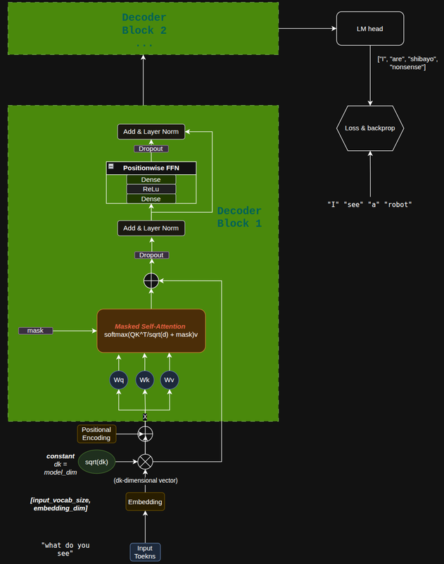
A real model stacks many of these blocks:
1
2
3
4
5
6
7
8
9
10
11
12
13
Embedding
    ↓
Decoder Block 1
    ↓
Decoder Block 2
    ↓
Decoder Block 3
    ↓
   ...
    ↓
Decoder Block N
    ↓
LM Head
5. The LM Head
The decoder does not directly output a word such as "robot".
It outputs a hidden vector:
\[h\in\mathbb{R}^{d_{\text{model}}}.\]The language-model head, or LM head, converts this hidden representation into one score for every token in the vocabulary.
For example, if
\[d_{\text{model}}=768\]and the vocabulary contains
\[|\mathcal V|=50{,}000\]tokens, the LM head performs a linear projection:
\[z = hW_{\text{vocab}} + b\]with
\[W_{\text{vocab}} \in \mathbb{R}^{768\times50{,}000}\]if \(h\) is represented as a row vector.
Thus:
1
2
3
4
5
6
7
8
9
10
11
hidden vector h
      ↓
   LM head
      ↓
50,000 logits

"The"       8.1
"robot"     4.7
"banana"   -1.2
"I"         7.8
...
Softmax converts these logits into probabilities:
\[P(w_i) = \frac{e^{z_i}} {\sum_j e^{z_j}}.\]During training, the correct next token determines the cross-entropy loss.
For example, if the correct answer is "I",
The model may currently predict "You" as its highest-probability token, but the training objective still pushes probability toward the ground-truth "I".
One useful implementation detail is weight tying (also in Series 5). Many language models reuse the token embedding matrix for the output LM head. Conceptually:
1
2
3
4
5
6
7
8
9
              shared weights
                    │
       ┌────────────┴────────────┐
       ▼                         ▼

token ID                    hidden state
   │                            │
   ▼                            ▼
embedding vector          vocabulary logits
This reduces the number of parameters and ties the input and output token representations together. It is common, although not mandatory.
Inference with KV Cache
During inference, there is no teacher correction. The model starts from the prompt, generates one token, appends that token to the context, and continues autoregressively until it generates an <EOS> token or another stopping condition is reached.
Without optimization, we could feed the entire growing sequence back through the Transformer every time. KV caching avoids most of this repeated computation.
Step 1: Process the prompt
Suppose, for simplicity, the prompt tokenizes into four tokens:
1
[x1, x2, x3, x4]
For each decoder layer, we calculate
\[Q=XW_Q,\qquad K=XW_K,\qquad V=XW_V.\]Therefore,
\[K= \begin{bmatrix} k_1\\ k_2\\ k_3\\ k_4 \end{bmatrix}, \qquad V= \begin{bmatrix} v_1\\ v_2\\ v_3\\ v_4 \end{bmatrix}.\]Attention is computed as
\[\operatorname{Attention}(Q,K,V) = \operatorname{softmax} \left( \frac{QK^T}{\sqrt{d_k}}+M \right)V,\]1
2
3
4
KV cache:
K_cache = [k1, k2, k3, k4]
V_cache = [v1, v2, v3, v4]
This initial processing of the whole prompt is often called prefill.
Step 2: Generate the next token
Conceptually, the sequence is now:
1
"What do you see? I"
Without KV caching, we could recompute:
\[K= [k_1,k_2,k_3,k_4,k_5]\]and
\[V= [v_1,v_2,v_3,v_4,v_5]\]from scratch.
But \(k_1,\ldots,k_4\) and \(v_1,\ldots,v_4\)have not changed. Therefore, with a KV cache, we feed only the newly generated token "I" through the model.
Why cache K,V, but not Q?
For the next generated token, we only need the new query.
For example, to generate token 6, we calculate \(q_6\) and ask:
\[\text{"How much should token 6 attend to every previous token?"}\]That requires
\[q_6k_1^T,\quad q_6k_2^T,\quad \dots,\quad q_6k_6^T.\]The old queries \(q_1,\ldots,q_5\) have already done their job. We do not need them again.