1. Problem Setup and Definitions
Imagine we now have a bunch of particles in the 1D world. They are all moving randomly. Along x axis, its current distribution can be characterized as a source distribution; 1s later, they scattered at a target distribution.
- The number of particles at position $x$ at time $t$ is called probability density, $p_t(x)$.
- The rate of change at a specific location
xis called probabity current, $j_t(x)$. That is, how much probability flows across $x$ per second. You can think of that as water current: some water (particles) flow in, some water flows out. - The lowest cost way to move particles to the target distribution is called Optimal Transport, or OT.
- Each particle has a velocity $v$. Laying all these particles’ velocities together will give us a velocity field
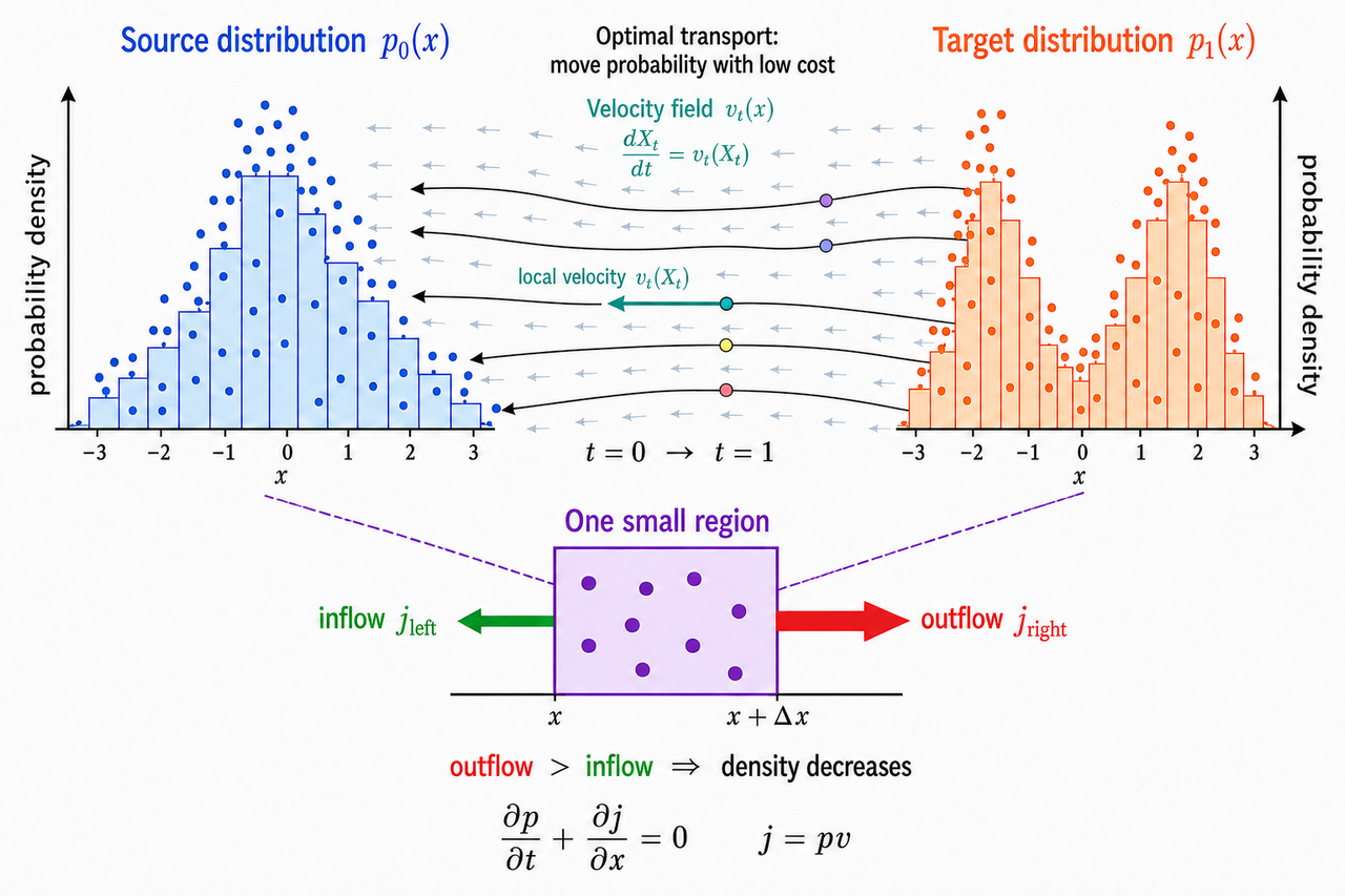
First, we know total probability is always 1. Particles (probability) flows from one location then flows in another.
\[\int_{-\infty}^{\infty} p_t(x)\,dx = 1.\]and
\[\int_{-\infty}^{\infty} \frac{\partial p_t(x)}{\partial t}\,dx = 0.\]Second is continuity equation - particles (probability) inside a small region can change only because probability flows through its boundaries. So it can’t disappear at one place and reappear at another without crossing the boundary:
\[\frac{\partial p_t(x)}{\partial t} + \frac{\partial j_t(x)}{\partial x} = 0\]In multiple dimensions, $\frac{\partial j}{\partial x}$ becomes divergence $\nabla \cdot j$
1-1 Explanation of The Above Using A Numerical example
Consider a box of width
\[\Delta x = 1\text{ m}.\]Suppose it initially contains probability $0.30$.
During the next $0.1$ seconds:
-
Incoming current on the left: $j_{\text{left}} = 0.08/\text{s}$
-
Outgoing current on the right: $j_{\text{right}} = 0.13/\text{s}$
The amounts moving during $0.1$ seconds are
\[P_{\text{in}} = 0.08(0.1) = 0.008,\]and
\[P_{\text{out}} = 0.13(0.1) = 0.013.\]Therefore, the box loses
\[\Delta P = 0.008 - 0.013 = -0.005.\]Its probability becomes
\[0.30 - 0.005 = 0.295.\]The density’s rate of change is
\[\frac{\partial p}{\partial t} \approx \frac{-0.005}{(1)(0.1)} = -0.05\frac{1}{\text{m}\cdot\text{s}}.\]Meanwhile, the current increases from $0.08$ to $0.13$ across the box:
\[\frac{\partial j}{\partial x} \approx \frac{0.13-0.08}{1} = 0.05\frac{1}{\text{m}\cdot\text{s}}.\]Thus,
\[\frac{\partial p}{\partial t} + \frac{\partial j}{\partial x} = -0.05 + 0.05 = 0.\]This means:
- More probability flowing out than in $\Rightarrow$ density decreases.
- More probability flowing in than out $\Rightarrow$ density increases. For the whole space,
If no probability escapes at infinity, then
\[j_t(\infty)=j_t(-\infty)=0.\]Therefore,
\[\frac{d}{dt} \int_{-\infty}^{\infty}p_t(x),dx = 0,\]so the total probability remains equal to $1$.
1-2 Another Definition of Probablity Current: $j_t(x)=p_t(x)v_t(x)$
Probability current means
\[\text{current} = \text{probability density} \times \text{net velocity at location}.\]Suppose that near position $x$,
\[p_t(x)=0.30/\text{m}, \qquad v_t(x)=2\text{ m/s}.\]In $0.1$ seconds, the particles travel
\[v\Delta t = 2(0.1) = 0.2\text{ m}.\]Therefore, the probability initially within $0.2$ m of the boundary crosses it. That probability is
\[\Delta P = p(v\Delta t) = (0.30)(0.2) = 0.06.\]The probability crossing the boundary per second is
\[j = \frac{\Delta P}{\Delta t} = \frac{0.06}{0.1} = 0.60/\text{s} = pv.\]Therefore, the flow-matching continuity equation is
\[\boxed{ \frac{\partial p_t(x)}{\partial t} + \nabla_x \cdot \left(p_t(x)v_t(x)\right) = 0 }\]In flow matching, the learned velocity field $v_t(x)$ moves each sample $X_t$ according to
\[\frac{dX_t}{dt} = v_t(X_t).\]2. Why Flow Matching Works
2-1. A Small Example
$p_t$ really is a path. if we have two paths, $p_{1t}$ and $p_{2t}$, at time t and location $x=5$, $p_{1t}$ has 60%, with $\text{net velocity} = -2/s$, $p_{2t}$ has 20%, with $\text{net velocity} = +1/s$. If you sum up all path’s probability current, probability density, you can find that velocity is the weighted average velocity: $0.6*-2 + 0.4 * 1 = -0.8/s$
Interesting thing is that when minimizing mean square error, we will get this average velocity. Assuming a is the final weighed average velocity the model outputs at $x=5$:
\[L(a) = 0.6(a- (-2))^2 + 0.4(a-1)^2\]Take derivative w.r.t $a$:
\[\frac{dL}{da} = 1.2(a+2) + 0.8(a-1) = -0.8\]So after a large number of training, MSE will make sure velocity output to be the weighted average.
2.2 Machine Learner Can Learn A Loss That’s Equivalent To the Optimum
In an ideal world, the optimal path velocity field is $u_t(x)$, at any state $x$ at time t. time $t \in [0,1]$ The loss of any velocity field output from the network is:
In a neural network, we don’t really have $u_t(x)$. We have our training targets, which is the end state at $t=1$, so the velocity field at $t$ is a conditional one: $u_t(x \mid X_1)$. So we are able to calculate $L_{CFM}$. For a random endpoint $x_1$, after observing that the path current state is $X=x$, the probability of ending at $x_1$ is $P_t(x_1 \mid x)$.
Then, we choose the optimal velocity to be
\[u_t(x) = \int u_t(x \mid X_1) P_1(X_1 \mid x)\,dX_1\]Meaning, the net optimal velocity at the given state $x$ is a weighted sum of all velocities $u_t(x \mid X_1)$ over their end states $X_1$, given the current state $x$. Note that at the same time $t$, multiple paths can pass through the same current state $x$ while ending at different $X_1$ values.
Using Bayes rule,
\[P_1(X_1 \mid x) = \frac{P_t(x \mid X_1) P_1(X_1)}{P_t(x)}\]Because $p_t(x)$ doesn’t depend on $d X_1$, we get:
\[\begin{aligned} & u_t(x) = \int \frac{u_t(x \mid X_1) P_t(x \mid X_1) P_1(X_1)}{P_t(x)}\,dX_1 \\ & = \frac{1}{P_t(x)} \int u_t(x \mid X_1) P_t(x \mid X_1) P_1(X_1)\,dX_1 \end{aligned}\]Using the definition of probability current
\[j_t(x \mid X_1) = u(x \mid X_1) p(x \mid X_1)\]We add up all contributions of each end point $X_1$ and get the overall probability current:
\[j_t(x) = \int u(x \mid X_1) p(x \mid X_1) p(X_1)\,dX_1\]Then we can conclude that the overall velocity :
\[u_t(x) = j_t(x) P_t(x)\]2-3. Conditional Flow Matching Loss is Equivalent to Flow Matching Loss
From the above, $u_t$ is ultimately the conditional optimal velocity field, $u_\text{cond}$. Of course,
\[\begin{aligned} & E[u_{cond}] = \int u_t(x \mid x_1) p_t(x_1 \mid X_T = x)\,dx_1 = u_t \\ & \Rightarrow \\ & E[u_{cond} - u_t] = 0 \end{aligned}\]The CFM loss is:
\[\begin{aligned} & L_{CFM} = E(|v_\theta (x) - u_{cond}(x)|^2) \\ & = E(|(v_\theta (x) - u_t) + (u_t - u_{cond}(x))|^2) \\ & = E(|(v_\theta (x) - u_t)|^2) + 2 * E[(v_\theta (x) - u_t)^T (u_t - u_{cond}(x))] + E[|u_{cond} - u_t|^2] \end{aligned}\]At a given $t$ and state $x$, our model velocity output is a constant. $u_t$ is also constant. So,
\[\begin{aligned} & E[(v_\theta (x) - u_t)^T (u_t - u_{cond}(x))] \\ & = (v_\theta (x) - u_t)^T E(u_t - u_{cond}(x)) \\ & = 0 \end{aligned}\]| And $E[ | u_{cond} - u_t | ^2]$ is a term that is not dependent on model parameters $\theta$, so the above written in the FM loss form becomes |
This is almost identical to the conditional flow-matching loss, so we use the flow-matching loss.
OT (Optimal Transport) pairing
The goal at this step is to pair up $x_0$ and $x_1$, so we can find conditional velocity $u_t(x \mid X_1)$ at each training step. An example in image generation is to pair up Gaussian noise with final cat or dog images.
Optimal Transport is to pair so minimum $\text{total velocity}^2$ is achieved . Without OT, assume:
X₀ ∈ {0, 10}. X₁ ∈ {2, 9}. One way to pair is 0 → 9,10 → 2. The velocities are 9 − 0 = +9, 2 − 10 = −8. Total squared velocities are 9² + (−8)²= 145. Also note that the two paths also intersect at t = 10/17. So if training lands at that point, we get two valid yet opposite directions to follow. The network would learn a weighted average of the two velocities, which may lead to a less-optimal result.
With OT, we find the pairing with minimum total squared velocities: 0 → 2,10 → 9. Total velocities are: 2² + (−1)²=5. In the meantime the two paths do not intersect, so we are minimizing chance of having multiple valid directions at a certain intermediate point.
Concentration of Measure
The concentration of measure phenomenon says that, under suitable conditions, a well-behaved random quantity in high dimensions is likely to be close to its typical value.
Consider (n) independent fair coin tosses. Represent the result as an (n)-dimensional vector:
\[\mathbf X=(X_1,\ldots,X_n),\]where
\[X_i= \begin{cases} 1, & \text{heads},\ 0, & \text{tails} \end{cases}\]For each toss,
\[\mathbb E[X_i]=\frac12=\mu.\]Because (X_i) is either (0) or (1), we have
\[X_i^2=X_i.\]Therefore,
\[\mathbb E[X_i^2]=\mathbb E[X_i]=\frac12.\]The variance of one toss is
\[\begin{aligned} \operatorname{Var}(X_i) &=\mathbb E[X_i^2]-\mathbb E[X_i]^2\ &=\frac12-\left(\frac12\right)^2\ &=\frac14. \end{aligned}\]After (n) tosses, the observed average heads is
\[\bar X=\frac1n\sum_{i=1}^n X_i.\]Its expected value is
\[\mathbb E[\bar X]=\frac12.\]However, the actual value of ($\bar X$) need not equal (1/2) in a particular experiment.
The variance of the fraction of heads is
\[\operatorname{Var}(\bar X) = \mathbb E\left[(\bar X-\mu)^2\right].\]Since
\[\bar X-\mu = \frac1n\sum_{i=1}^n(X_i-\mu).\]we obtain
\[\begin{aligned} \operatorname{Var}(\bar X) &= \mathbb E\left[ \left( \frac1n\sum_{i=1}^n(X_i-\mu) \right)^2 \right]\ &= \frac1{n^2} \mathbb E\left[ \left( \sum_{i=1}^n(X_i-\mu) \right)^2 \right]. \end{aligned}\]Expanding the squared sum gives
\[\left( \sum_{i=1}^n(X_i-\mu) \right)^2 = \sum_{i=1}^n(X_i-\mu)^2 + 2\sum_{i<j}(X_i-\mu)(X_j-\mu).\]The cross terms have a plus sign. Because different tosses are independent,
\[\begin{aligned} \mathbb E[(X_i-\mu)(X_j-\mu)] &= \mathbb E[X_i-\mu] \mathbb E[X_j-\mu]\ &=0\cdot0\ &=0 \end{aligned}\]for ($i\neq j$).
Therefore, the cross terms vanish after taking the expectation. We are left with
\[\begin{aligned} \operatorname{Var}(\bar X) &= \frac1{n^2} \sum_{i=1}^n \mathbb E[(X_i-\mu)^2]\ &= \frac1{n^2} \sum_{i=1}^n \operatorname{Var}(X_i)\ &= \frac1{n^2} \left(n\cdot\frac14\right)\ &= \frac1{4n}. \end{aligned}\]Therefore, the standard deviation of the fraction of heads is
\[\operatorname{std}(\bar X) = \sqrt{\frac1{4n}} = \frac1{2\sqrt n}.\]As (n) increases, this standard deviation approaches zero. Consequently, the observed fraction of heads becomes increasingly concentrated around (1/2).
What happens to the vector’s ($L^2$) norm?
The squared $L^2$ norm of the binary vector is
\[\begin{aligned} |\mathbf X|_2^2 &= \sum_{i=1}^nX_i^2\ &= \sum_{i=1}^nX_i\ &= n\bar X. \end{aligned}\]Because ($\bar X$) is usually close to (1/2),
\[|\mathbf X|_2^2\approx\frac n2.\]Therefore,
\[|\mathbf X|_2\approx\sqrt{\frac n2}.\]The $L^2$ norm does not decrease as the dimension increases. It grows approximately like ($\sqrt{n/2}$).
However, for a fixed large dimension (n), most randomly generated coin-toss vectors have similar $L^2$ norms because most contain approximately (n/2) ones.
Equivalently, the normalized norm concentrates:
\[\frac{|\mathbf X|_2}{\sqrt n} \approx \frac1{\sqrt2}.\]This is the concentration effect: the vectors do not become small, but their norms become increasingly similar relative to their overall scale.
Q&A
- does velocity need to be a unit vector? No
- is it suitable for generating noisy seabed, because the same seabed could have different noisy outputs? flow matching sounds like a deterministic network to me. Or in one of your points, we are learning the expected velocity, at a specific time t.