## 1. What continual learning actually means

Suppose a detector is trained on Dataset 1. Later, Dataset 2 arrives. We want to train on Dataset 2 without keeping all of Dataset 1 in every training run—and without destroying performance on Dataset 1. That is the central problem of continual learning.

Continual learning asks what knowledge survives a sequence of training experiences.

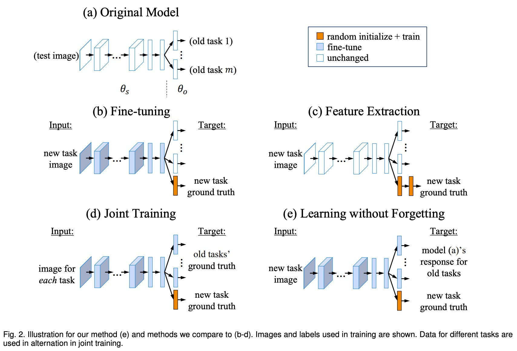
Ordinary supervised learning assumes that training examples are sampled from a more or less fixed distribution. Continual learning replaces that assumption with a stream of experiences:

\[\mathcal{D}_1 \rightarrow \mathcal{D}_2 \rightarrow \cdots \rightarrow \mathcal{D}_T.\]

After learning experience $t$, we evaluate the model not only on the newest distribution, but on all distributions seen so far. If learning $\mathcal{D}_2$ reduces performance on $\mathcal{D}_1$, the model has experienced negative backward transfer. Severe negative backward transfer is called catastrophic forgetting.

The key tension is:

Plasticity: learn the new data well.
Stability: preserve useful behavior learned from old data.

Excessive plasticity causes forgetting. Excessive stability prevents adaptation.

Continual-learning papers often distinguish three settings:

Task-incremental learning: the task identity is known at inference. The system may select a task-specific head or adapter.
Domain-incremental learning: the task stays the same, but the input distribution changes—for example, close-range sonar versus far-range sonar.
Class-incremental learning: new classes arrive over time, and inference must choose among all classes without being told which learning phase an input came from.

These settings are not interchangeable. Separate LoRA adapters are much easier to use when a reliable task or domain identifier is available. They are less satisfying when the model must infer the domain and class in one pass.

2. Why sequential fine-tuning forgets

Let the model parameters after Dataset 1 be $\theta_1$. When we fine-tune only on Dataset 2, gradient descent optimizes

\[\min_\theta \; \mathcal{L}_2(\theta).\]

Nothing in this objective requires $\mathcal{L}_1(\theta)$ to remain small. If the gradients that improve Dataset 2 point against directions important for Dataset 1, the new optimization step damages old behavior.

This is not merely “the model running out of memory.” The model may have ample parameter capacity. The problem is that Dataset 2 provides no evidence about which old behaviors must remain invariant. Here is a family of methods that address this issue:

Family	Core idea	Main cost or limitation
Replay or rehearsal	Mix stored old examples with new examples	Retains data; buffer selection matters
Generative replay	Generate approximations of old examples	Generator can drift or omit rare cases
Regularization	Penalize changes to parameters important to old tasks	Importance estimates are approximate; can restrict learning
Distillation	Keep the new model’s old-task outputs close to the previous model	Preserves previous predictions, including errors
Gradient constraints	Reject or project updates that would harm remembered old data	Additional gradient computation
Parameter isolation	Give new tasks separate modules, heads, or subnetworks	Model storage grows; routing may be required
Dynamic expansion	Add capacity as tasks arrive	Growing deployment and maintenance cost

Elastic Weight Consolidation (EWC), for example, adds a penalty for moving parameters considered important to previous tasks:

\[\mathcal{L}(\theta) = \mathcal{L}_2(\theta) + \frac{\lambda}{2} \sum_i F_i(\theta_i-\theta_{1,i})^2,\]

where $F_i$ approximates the importance of parameter $i$. Gradient Episodic Memory (GEM) instead stores examples from old tasks and constrains new gradients so that the remembered losses do not increase.

In practical computer-vision systems, a small, representative replay buffer is often the baseline to beat. It directly supplies the missing evidence: “these old examples still matter.”

3. What LoRA (Low Rank Adaptation) changes mathematically

Consider a pretrained weight matrix

\[W_0 \in \mathbb{R}^{d_{\text{out}}\times d_{\text{in}}}.\]

Full fine-tuning learns an unrestricted update $\Delta W$ with the same shape. LoRA freezes $W_0$ and parameterizes the update as

\[W_{\text{eff}} = W_0+\frac{\alpha}{r}BA,\]

where A and B are two smaller matrices (so fewer parameters to learn)

$A\in\mathbb{R}^{r\times d_{\text{in}}}, \qquad B\in\mathbb{R}^{d_{\text{out}}\times r}, \qquad r\ll\min(d_{\text{in}},d_{\text{out}}).$ Because

\[\operatorname{rank}(BA)\le r,\]

LoRA restricts the update to a low-rank form. Instead of training $d_{\text{out}}d_{\text{in}}$ parameters, it trains

\[r(d_{\text{in}}+d_{\text{out}})\]

parameters for that weight.

For a convolution,

\[W_0\in \mathbb{R}^{C_{\text{out}}\times C_{\text{in}}\times k_h\times k_w},\]

one conceptual view is to flatten it into

\[W_0\in \mathbb{R}^{C_{\text{out}}\times(C_{\text{in}}k_hk_w)}\]

and apply the same factorization.

LoRA provides three important engineering benefits:

The large base weights remain frozen.
Optimizer states and gradients are stored only for the small adapter parameters.
The learned update can often be merged into the base weight for inference.

The original LoRA paper demonstrated these advantages for large Transformer models. They are most valuable when the base model is large. On a small 2.2-million-parameter U-Net, LoRA may save less than the added system complexity is worth.

4. Why LoRA does not automatically prevent forgetting

There are three different designs that people casually call “continual learning with LoRA.” They behave very differently.

Design A: Reuse one LoRA adapter

Train adapter parameters $(A,B)$ on Dataset 1, then continue updating the same parameters on Dataset 2.

This is simply sequential fine-tuning inside a smaller parameter space. The base weight $W_0$ is protected, but the adapter’s Dataset-1 update can still be overwritten. The detector head can also forget if it remains trainable.

LoRA may reduce interference because it limits the update space. It can also increase interference if multiple tasks compete for the same low-rank directions. There is no general guarantee either way.

Design B: Add one adapter per dataset or domain

Keep $(A_1,B_1)$ for Dataset 1 frozen, then learn a new $(A_2,B_2)$ for Dataset 2. Direct parameter overwriting is avoided. But now, how do we choose or combine outputs?. If task identity is supplied, this is task-incremental learning. If a router predicts the domain, overall performance depends on routing accuracy. If all adapters are simply summed,

\[W_{\text{eff}} = W_0+\sum_{t=1}^{T}B_tA_t,\]

the combined update has rank at most $\sum_t r_t$, but that does not mean the adaptations are compatible. Their functional effects can conflict. Storage also grows approximately linearly with the number of tasks.

Design C: Use LoRA inside an actual continual-learning algorithm

Recent methods combine low-rank adaptation with replay, gradient-subspace constraints, orthogonal updates, regularization, or adapter selection. For example, InfLoRA attempts to place new low-rank updates in directions that avoid old-task gradient subspaces. CL-LoRA addresses rehearsal-free class-incremental learning with additional mechanisms beyond ordinary LoRA.

The important phrase is beyond ordinary LoRA. The continual-learning behavior comes from the replay, routing, projection, regularization, or isolation rule—not from low rank alone.

Summary

Method	Training sequence	What it diagnoses
Joint-training oracle	Shuffle Datasets 1 and 2 together	Best attainable result with full data access
Sequential full fine-tuning	Dataset 1, then Dataset 2	Amount of ordinary forgetting
Sequential shared LoRA	Dataset 1, then Dataset 2 using one adapter	Whether low-rank restriction alone helps
Separate routed LoRAs	One frozen adapter per range regime	Value of parameter isolation plus routing
Shared LoRA + replay	Dataset 2 plus a small Dataset-1 buffer	Whether remembered examples solve the main interference

A useful forgetting score for Domain 1 is

\[F_1 = R_{1,1}-R_{2,1}.\]

Positive $F_1$ means the model forgot Domain 1 after learning Domain 2. Also report final average performance:

\[\text{FinalAvg} = \frac{R_{2,1}+R_{2,2}}{2}.\]

5. Common misconceptions

“A separate LoRA for every dataset means the model remembers everything”

It preserves each adapter, assuming the corresponding head and preprocessing are also preserved. It does not solve routing or integrate the knowledge. In the meantime, Matrix addition is easy; behavioral compatibility is not guaranteed. The merged model must be evaluated on every old and new domain.

So, Run an experiment first. LoRA is a plausible implementation tool but not yet the leading solution.

“Low rank means tasks cannot interfere”

Low rank limits the update space. Two tasks can still want incompatible changes inside that space.

2 - AdaBN: Domain Adaptation Without Retraining the Network

Machine-learning models often perform well on data that resembles their training set and then degrade when the input distribution changes. A camera changes, a sensor gain drifts, weather becomes worse, or synthetic training data gives way to real measurements. The task may be unchanged, but the model’s internal activations no longer look like the activations it learned to process.

Adaptive Batch Normalization, or AdaBN, addresses one narrow but useful part of this problem. It replaces BatchNorm statistics learned from the source domain with statistics measured from unlabeled target-domain data. It does not retrain the convolution weights, and classical AdaBN does not optimize a loss.

That simplicity is AdaBN’s main advantage—and its main limitation.

2-1 BatchNorm during training and inference

For one activation channel, BatchNorm applies

\[y = \gamma\frac{x-\mu}{\sqrt{\sigma^2+\epsilon}}+\beta.\]

The four quantities play different roles:

$\mu$ and $\sigma^2$ describe the activation distribution.
$\gamma$ and $\beta$ are learned scale and bias parameters.

During training, BatchNorm calculates a mean and variance from each mini-batch. It also maintains running estimates of these statistics. During ordinary inference, the running statistics are frozen and reused for every input. The inference data does not normally change them. This works when training and deployment data have similar distributions. Under domain shift, however, the stored source statistics may normalize target activations badly.

2-2 The central idea of AdaBN

Assume that a model was trained on a source domain and will be deployed on a related target domain. Classical AdaBN performs four steps:

Freeze the learned network weights.
Pass unlabeled target samples through the network.
Estimate a target mean and variance for every BatchNorm channel.
Replace the source running statistics $\mu$ and $\sigma$ with the target statistics.

The new inference equation becomes

\[y = \gamma\frac{x-\mu_{\text{target}}} {\sqrt{\sigma^2_{\text{target}}+\epsilon}}+\beta.\]

The learned $\gamma$, $\beta$, convolution weights, and prediction heads remain unchanged. No target labels are required.

2-3 Offline AdaBN

Offline AdaBN assumes that a representative set of unlabeled target data is available before deployment.

The workflow is:

Save the original source model.
Run a target calibration set through it without gradients.
accumulate BatchNorm moments across the calibration set;
save the resulting target statistics as a new model state;
return the model to evaluation mode and freeze those statistics.

One can stop updating AdaBN when both the BatchNorm statistics and validation metrics become stable.

2-4 Online AdaBN and prediction-time normalization

“Online AdaBN” is best treated as an extension of the classical method, not as the only canonical form of AdaBN. Related literature often uses names such as prediction-time BatchNorm, test-time normalization, or online test-time adaptation.

The online idea is simple: update the running target statistics as new unlabeled inputs arrive.

For an exponential update,

\[\mu_t=(1-\alpha)\mu_{t-1}+\alpha\hat{\mu}_t,\] \[\sigma_t^2=(1-\alpha)\sigma_{t-1}^2+\alpha\hat{\sigma}_t^2,\]

where $\hat{\mu}_t$ and $\hat{\sigma}_t^2$ are statistics from the new data and $\alpha$ controls adaptation speed.

The approximate half-life of past information is

\[h=\frac{\ln(0.5)}{\ln(1-\alpha)}.\]

$\alpha$	Approximate half-life
0.001	693 updates
0.01	69 updates
0.1	7 updates

A large $\alpha$ adapts quickly but can be corrupted by a short unusual sequence. A small $\alpha$ is stable but may respond too slowly to real drift.

Why online adaptation is risky

Online AdaBN adds state to the model. The prediction is no longer a function of the current input alone:

\[\hat{y}_t=f(x_t,s_{t-1}),\]

where $s_{t-1}$ contains the accumulated BatchNorm statistics.

This creates several failure modes:

Temporal correlation: many nearly identical inputs can dominate the state.
Abrupt transitions: the distribution can change faster than a slow update follows it.
Transient contamination: an unusual event can shift statistics for later predictions.
Order dependence: shuffling the same inputs can change the result.
Silent degradation: there may be no label or loss signal indicating that adaptation is moving in the wrong direction.

A practical online system should retain an immutable fallback state, reset at clear boundaries, log statistic drift, and use an update rate chosen on chronological validation sequences.

2-5 What AdaBN can and cannot fix

AdaBN is most plausible when the task remains the same but internal feature moments shift.

It may help with:

broad sensor gain or contrast changes;
changed average feature magnitude;
changed channel variance;
moderate covariate shifts represented in the calibration data.

It cannot reliably fix:

missing classes or unseen object structures;
multimodal target distributions that one mean and variance represent poorly.

Start with offline AdaBN. It is the cheapest and most interpretable experiment. Test online updates only when the target distribution genuinely changes over time and offline statistics become stale.

The correct mental model is modest:

AdaBN does not teach the network a new task. It changes the coordinate system in which the existing network interprets the new domain.

[ML] Continual Learning

LoRA, AdaBN