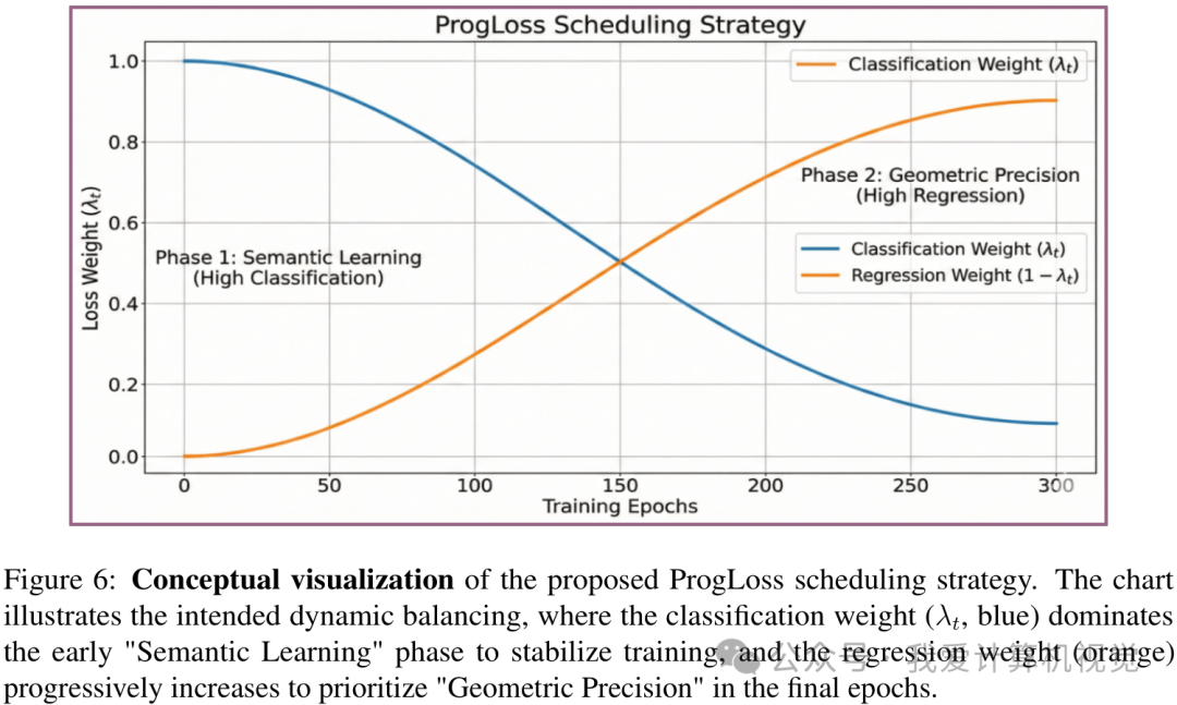
ProgLoss is a training-time loss schedule for object detection. Instead of keeping classification and localization weights fixed for all epochs, it changes them over training progress:
\[L_{\operatorname{total}}(t) = \lambda_{\operatorname{cls}}(t)L_{\operatorname{cls}} + \lambda_{\operatorname{box}}(t)L_{\operatorname{box}}.\]Early training emphasizes classification; later training emphasizes localization. This progressive shift is described in YOLO26 discussions of ProgLoss. (Ultralytics)
1. Basic detection loss
A YOLO-style detector usually has a loss like:
\[L = \lambda_{\operatorname{cls}}L_{\operatorname{cls}} + \lambda_{\operatorname{box}}L_{\operatorname{box}} + \lambda_{\operatorname{obj}}L_{\operatorname{obj}}.\]For a modern anchor-free detector, you can simplify it as:
\[L = \lambda_{\operatorname{cls}}L_{\operatorname{cls}} + \lambda_{\operatorname{box}}L_{\operatorname{box}}.\]ProgLoss makes the weights time-dependent:
\[L(t)=\lambda_{\mathrm{cls}}(t)L_{\mathrm{cls}}+\lambda_{\mathrm{box}}(t)L_{\mathrm{box}}.\]2. A simple ProgLoss schedule
Let training progress be
\[p = \frac{t}{T}\]where:
\[t = \text{current epoch}\] \[T = \text{total epochs}\]So:
\[p=0\]means training just started, and
\[p=1\]means training is finished.
A simple linear schedule is:
\[\lambda_{\text{cls}}(p) = 1 - p\] \[\lambda_{\text{box}}(p) = p\]But this becomes zero at the endpoints, which may be too aggressive. A safer version is:
\[\lambda_{\text{cls}}(p)=\lambda_{\text{cls,end}} + (\lambda_{\text{cls,start}}-\lambda_{\text{cls,end}})(1-p)\] \[\lambda_{\text{box}}(p)=\lambda_{\text{box,start}} + (\lambda_{\text{box,end}}-\lambda_{\text{box,start}})p\]Example:
\[\lambda_{\text{cls,start}}=2.0, \qquad \lambda_{\text{cls,end}}=0.5\] \[\lambda_{\text{box,start}}=0.5, \qquad \lambda_{\text{box,end}}=2.0\]Then:
\[\lambda_{\text{cls}}(p)=2.0-1.5p\] \[\lambda_{\text{box}}(p)=0.5+1.5p\]So the full loss is:
\[L(p) = (2.0-1.5p)L_{\text{cls}} + (0.5+1.5p)L_{\text{box}}.\]3. Small numeric example
Suppose we train for:
\[T = 100 \text{ epochs}\]and at one batch, the raw losses are:
\[L_{\text{cls}} = 0.8\] \[L_{\text{box}} = 0.4\]Use:
\[\lambda_{\text{cls}}(p)=2.0-1.5p\] \[\lambda_{\text{box}}(p)=0.5+1.5p\]Epoch 0
\[p = \frac{0}{100}=0\] \[\lambda_{\text{cls}}=2.0\] \[\lambda_{\text{box}}=0.5\]Therefore:
\[L = 2.0(0.8)+0.5(0.4)=1.8\]Early training is dominated by classification:
1
2
classification contribution = 1.6
box contribution            = 0.2
So the model focuses on learning what object is present.
Epoch 50
\[p = \frac{50}{100}=0.5\] \[\lambda_{\text{cls}}=2.0-1.5(0.5)=1.25\] \[\lambda_{\text{box}}=0.5+1.5(0.5)=1.25\]Therefore:
\[L = 1.25(0.8)+1.25(0.4)=1.5\]Now classification and localization are balanced.
Epoch 100
\[p = \frac{100}{100}=1\] \[\lambda_{\text{cls}}=0.5\] \[\lambda_{\text{box}}=2.0\]Therefore:
\[L = 0.5(0.8)+2.0(0.4)=1.2\]Late training is dominated by localization:
1
2
classification contribution = 0.4
box contribution            = 0.8
So the model focuses on refining where the object is.
4. Why this helps without DFL
DFL, or Distribution Focal Loss, helps box localization by predicting coordinate distributions instead of only direct box values. YOLO26 summaries say DFL is removed to simplify deployment/export and reduce overhead, while ProgLoss and STAL are introduced as training-time improvements to keep localization quality strong. (Datature)
So ProgLoss acts like a curriculum:
\[\text{early stage: semantic learning}\] \[\text{late stage: geometric refinement}\]This is useful because if box regression dominates too early, the detector may try to precisely localize objects before it has learned stable object/category features.
5. Slightly more realistic formulation
Usually the box loss may be IoU-based:
\[L_{\text{box}} = 1 - \operatorname{IoU}(B_{\text{pred}}, B_{\text{gt}})\]and classification may be BCE or focal loss:
\[L_{\text{cls}} = -\left( y\log(p)+(1-y)\log(1-p) \right).\]Then ProgLoss is:
\[L(t) = \lambda_{\text{cls}}(t) \left[-\left(y\log(p)+(1-y)\log(1-p)\right)\right] + \lambda_{\text{box}}(t) \left[1-\operatorname{IoU}(B_{\text{pred}},B_{\text{gt}})\right].\]At the beginning:
\[\lambda_{\text{cls}}(t) > \lambda_{\text{box}}(t)\]At the end:
\[\lambda_{\text{box}}(t) > \lambda_{\text{cls}}(t)\]6. Pseudocode
1
2
3
4
5
6
7
8
9
10
11
12
13
14
15
16
17
18
19
20
21
def progloss(
    cls_loss,
    box_loss,
    epoch,
    total_epochs,
    cls_start=2.0,
    cls_end=0.5,
    box_start=0.5,
    box_end=2.0,
):
    # progress from 0 to 1
    p = epoch / total_epochs

    # progressive weights
    lambda_cls = cls_start + (cls_end - cls_start) * p
    lambda_box = box_start + (box_end - box_start) * p

    # total detection loss
    total_loss = lambda_cls * cls_loss + lambda_box * box_loss

    return total_loss, lambda_cls, lambda_box
Training loop:
1
2
3
4
5
6
7
8
9
10
11
12
13
14
15
16
17
for epoch in range(total_epochs):
    for images, targets in dataloader:
        pred = model(images)

        cls_loss = classification_loss(pred, targets)
        box_loss = box_regression_loss(pred, targets)

        loss, lambda_cls, lambda_box = progloss(
            cls_loss=cls_loss,
            box_loss=box_loss,
            epoch=epoch,
            total_epochs=total_epochs,
        )

        optimizer.zero_grad()
        loss.backward()
        optimizer.step()
7. Summary
ProgLoss changes this:
\[L = \lambda_{\text{cls}}L_{\text{cls}}+\lambda_{\text{box}}L_{\text{box}}\]from fixed weights to dynamic weights:
\[L(t)=\lambda_{\text{cls}}(t)L_{\text{cls}}+\lambda_{\text{box}}(t)L_{\text{box}}.\]The purpose is:
\[\boxed{ \text{early: learn to classify} }\] \[\boxed{ \text{late: learn to localize precisely} }\]In plain language: ProgLoss first pushes the detector on what the object is, then gradually shifts emphasis to where the object is.