1. Tesla’s Perception Challenges (2021)
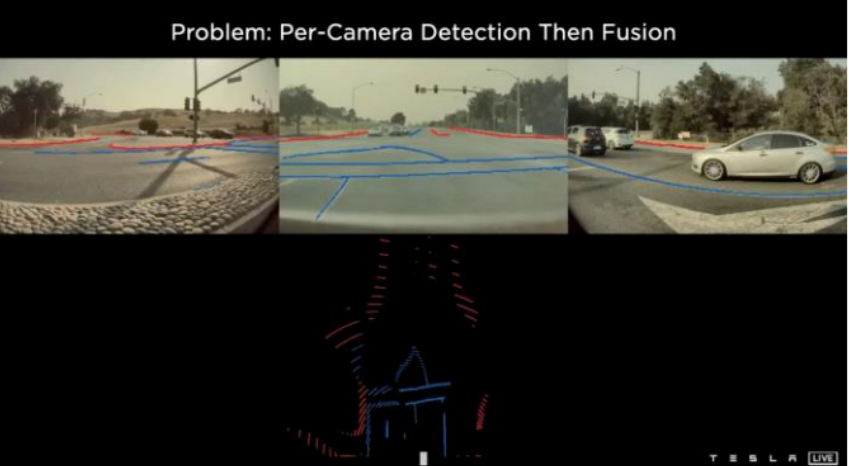
Before BEV, Tesla’s pipeline detected objects and lanes independently in each camera view and then tried to fuse the results. This created fundamental problems:
Lane detection was unreliable.
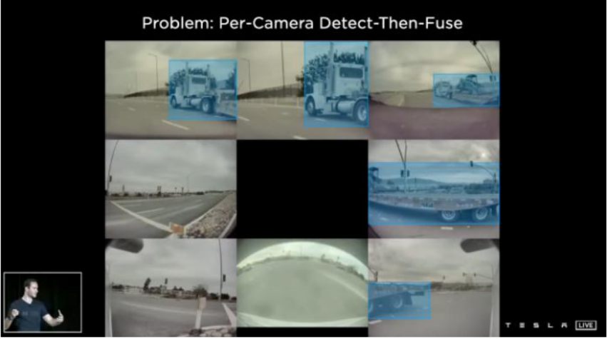
Per-camera detect-then-fuse breaks for large objects. If a truck spans multiple cameras, how do you tell which detections belong to the same object? Recovering the full 3D shape of a large vehicle from disjointed per-camera boxes is hard.
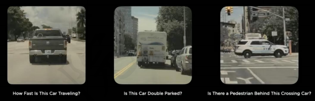
No shared spatial context. Each camera sees its own patch of the world. Questions like “how fast is that truck moving?”, “is it double-parked?”, and “is there a pedestrian behind it?” need a shared spatial frame to answer reliably.
Lane markings are hard to preserve across views and over time.
Tesla’s solution: Move to a unified top-down (“local map”) representation — a Bird’s Eye View (BEV). BEV provides a single, ego-centric spatial grid where features from all cameras can be fused in a common coordinate frame, and temporal accumulation is straightforward.
2. The Evolution of Tesla’s Vision Stack
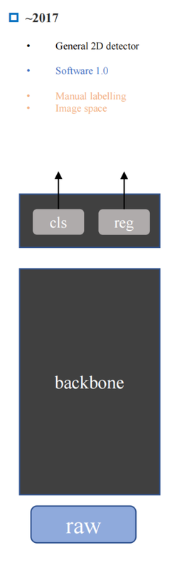
2017: Per-image range detection (regression) and classification. One model, one camera, one task at a time.
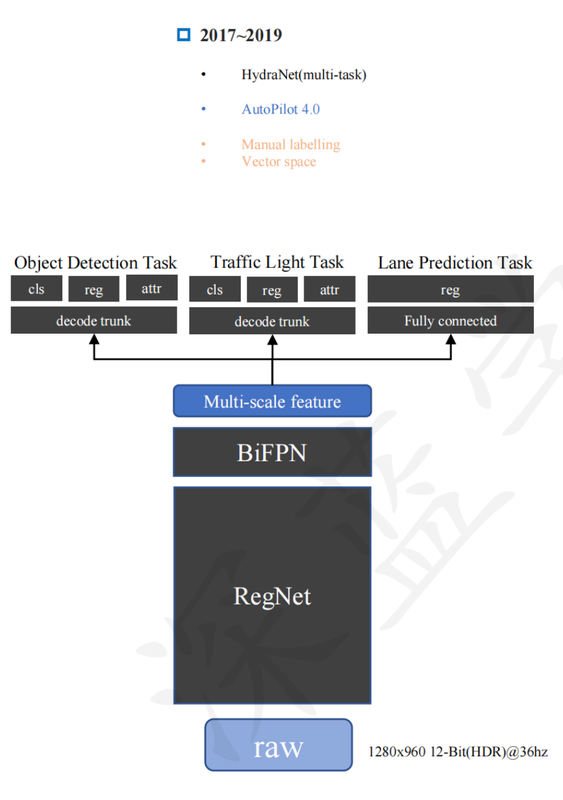
Later: Multi-camera, multi-task models. Several cameras feed into shared feature extractors; outputs include depth, segmentation, object detection simultaneously.
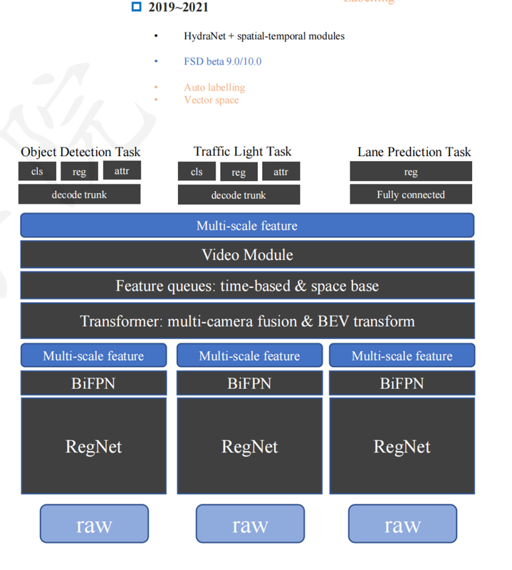
Vector Space / Feature Queue: Features are not just pooled but stored in a spatial queue across time. This supports:
- Spatial: merging overlapping camera fields of view into a consistent grid
- Temporal: accumulating features from past frames to handle occlusion and velocity estimation
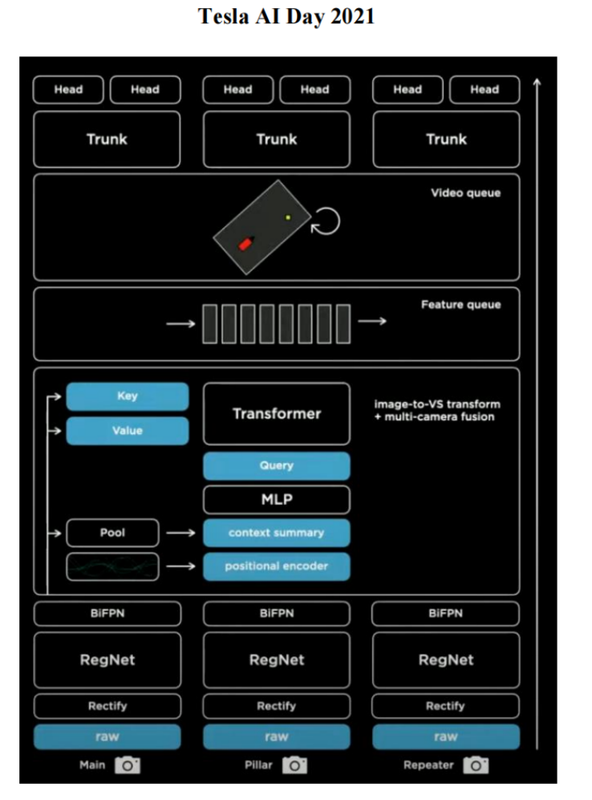
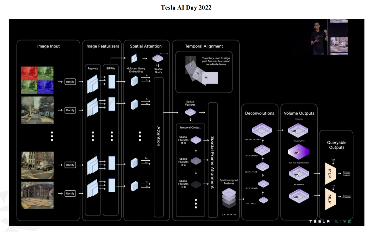
The transformer-based architecture works as follows:
- Take images from multiple cameras at multiple timesteps; rectify them
- Feed each image through an image feature extractor (backbone)
- Generate keys and values per image; generate a spatial BEV query over the shared grid
- Cross-attention produces BEV-aligned spatial features, all referenced to the same ego frame at time $T$
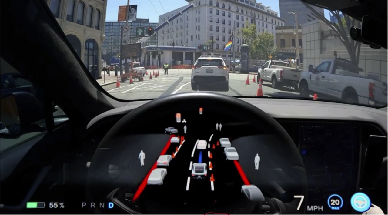
Tesla is notable for using no HD map — all spatial context is built on-the-fly from vision alone. Their data closed-loop (auto-labeling triggered by edge cases, retrain, redeploy) is a major competitive advantage. The system powers NOA (Navigate on Autopilot / Navigate on Autosteer) in city driving.
3. Tesla’s Full Perception Pipeline
Target: L2+ (and eventually FSD) perception from vision only.
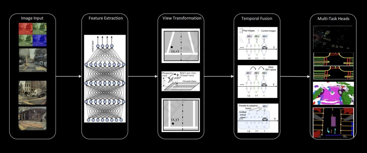
The pipeline has five stages:
| Stage | What it does |
|---|---|
| 1. Feature extraction | Each camera image passes through a backbone (e.g. ResNet, RegNet) to produce a rich feature map |
| 2. View transform | Image features are lifted from perspective views into a shared BEV / 3D vector space using cross-attention or geometric projection |
| 3. Spatial fusion | BEV features from all cameras are merged into a single ego-centric grid (Spatial Transformer, BEV) |
| 4. Temporal fusion | Consecutive BEV frames are aligned (using ego-motion) and fused to aggregate motion cues and reduce occlusion uncertainty |
| 5. Multi-task heads | The fused BEV representation feeds task-specific heads: occupancy grid, free-space, parking, lane geometry, object detection |
Why temporal fusion after spatial fusion? The spatial transform produces a BEV frame tied to a single timestep. Temporal fusion then aligns and merges multiple such BEV frames across time using ego-motion, which is easier and more principled in BEV space than in perspective image space.
4. Training a BEV Network: Where Does Ground Truth Come From?
Camera-only networks need depth or occupancy supervision, but depth sensors are either absent at inference time or intentionally excluded. The answer is an offline auto-labeling pipeline.
4.1 Offline Reconstruction Pipeline
Companies run a heavy reconstruction stack offline (after data collection, not in real time):
1
2
3
4
5
6
7
8
9
1. Collect: synchronized multi-camera video + calibration + ego-motion (GPS/IMU)
2. Reconstruct: run offline SLAM / SfM / MVS / bundle-adjustment stack
3. Label:  generate pseudo-ground-truth targets
             ├── 3D points / surfaces
             ├── object tracks and bounding boxes
             ├── occupancy volumes
             ├── lane geometry
             └── free-space masks
4. Train:  supervise online network to predict those targets from raw images alone
Depth output density varies by method:
| Output | Typical source |
|---|---|
| Sparse depth | SfM / feature matching |
| Semi-dense depth | Direct methods (LSD-SLAM, DSO) |
| Dense depth | Multiview stereo, depth completion |
| Surface estimates | TSDF fusion, mesh reconstruction |
4.2 Voxel Occupancy as Training Target
Rather than regressing metric depth per pixel, it is more useful to voxelize the scene:
- Occupied — a reconstructed surface or tracked object is present
- Free — a camera ray passed through without hitting anything
- Unknown — no ray coverage
This is task-aligned for autonomous driving and avoids single-pixel depth regression difficulties.
4.3 Feature Reprojection Loss (Self-Supervised Signal)
An additional signal needs no offline reconstruction:
- Predict depth or lifted 3D features from frame $t$
- Project them into another camera or frame $t+1$ using known ego-motion
- Compare against actual observations there (photometric or feature-level loss)
This is the basis of methods like Monodepth2 and SurroundDepth.
5. Multi-View Geometry: The Offline Reconstruction Stack
The offline pipeline is built on classical multi-view geometry, extended with dense methods:
5.1 Sparse Pipeline
1
2
3
4
5
1. Detect and match feature points (SIFT, SuperPoint, ORB, ...)
2. Apply epipolar geometry + RANSAC to filter bad matches
3. Recover relative camera poses from fundamental / essential matrix
4. Triangulate matched point pairs into 3D
5. Refine globally with bundle adjustment → sparse point cloud
Epipolar geometry and triangulation give the geometric skeleton.
5.2 Densification and Semantic Enrichment
| Technique | Output |
|---|---|
| Multiview stereo (MVS) | Dense depth / point cloud |
| Plane / surface fitting | Ground plane, facades |
| Temporal fusion | Consistent HD map across drives |
| Semantic segmentation | Per-voxel class labels |
| Object-level reconstruction | Tracked 3D bounding boxes |
The full pipeline densifies, cleans, and semantically organizes the skeleton into the rich training targets (lanes, curbs, occupancy volumes, tracked objects) that sparse SfM alone cannot provide.
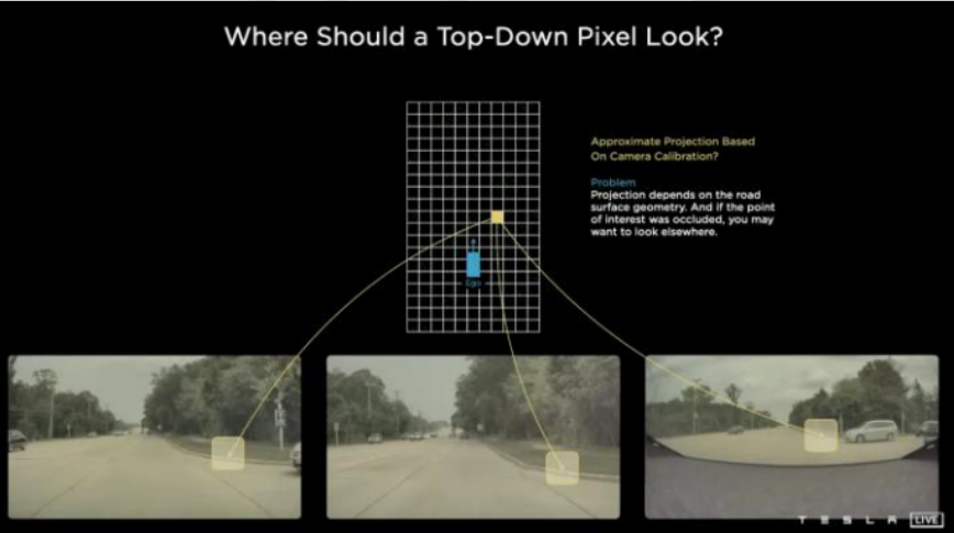
6. View Transformation: From Images to BEV
6.1 The Depth Ambiguity Problem
A single pixel $(u, v)$ maps not to one 3D point but to an entire ray:
\[\mathbf{p}_{3D} = \mathbf{o} + d \cdot \hat{\mathbf{r}}_{u,v}, \quad d \in [d_{\min}, d_{\max}]\]Without knowing $d$, you cannot assign that image feature to a unique BEV grid cell. This is the core difficulty of perspective-to-BEV lifting.
6.2 IPM — Inverse Perspective Mapping
IPM resolves the ambiguity by assuming all scene points lie on the ground plane ($Z = 0$). The constraint turns the projection into a planar homography — closed-form, no learning required.
- Good for: flat road surface, lane markings
- Bad for: vehicles, pedestrians, curbs, overpasses
6.3 Why Lift Features, Not Raw Pixels
| Warp pixels first | Warp features first |
|---|---|
| Heavy distortion and missing regions | Features already encode edges, objects, lanes |
| Backbone sees broken, unrealistic input | Backbone invariances (lighting, viewpoint) carry over |
Correct order:
1
image → backbone → feature map → geometric lifting → BEV fusion
6.4 Four Lifting Methods
| Method | Mechanism | Papers |
|---|---|---|
| A. IPM / flat-ground | Ground-plane homography; no depth network | Classic |
| B. Depth distribution | Predict softmax over depth bins; lift feature along ray | LSS, BEVDet |
| C. Cross-attention | BEV queries attend to image features; geometry in positional embeddings | BEVFormer, DETR3D, PETR |
| D. Occupancy prediction | Predict voxel occupancy directly; bypass explicit depth | MonoScene, TPVFormer |