Understanding L2 and L2+ Perception: Why the Real Challenge Is System Design, Not Just Better Detection
When people talk about assisted driving, they often jump straight to compute power, perception models, or the latest sensor stack. But in practice, L2 and L2+ systems are defined less by any single model and more by application constraints, feature scope, and how the full perception-to-decision chain is designed.
At a high level, the needs of the application determine the system. A typical L2 system requires less than 20 TOPS of compute and focuses on relatively structured environments such as highways and bridges. L2+ expands that scope, often adding features like automated lane changes and on-ramp or off-ramp assistance. Platforms from vendors like Nvidia can range from roughly 200 to 300 TOPS, giving ~1000 TOPS across multiple cards, but raw compute alone does not solve the core autonomy problem.
What L2 Usually Means in Practice
A basic L2 driving stack is typically built around a small set of core functions:
- LKA (Lane Keeping Assist) for keeping the vehicle centered in the lane
- ACC (Adaptive Cruise Control) for maintaining speed and following distance
- AEB (Automatic Emergency Braking) for emergency stopping when a collision risk is detected
In real deployments, these functions are rarely isolated. They depend heavily on the quality of lane perception, object detection, tracking, free-space understanding, and system-level fusion.
For L2+, the system often extends beyond simple lane centering and longitudinal control. Features like automatic lane changes or highway ramp handling introduce more edge cases, more rules, and more dependence on reliable scene understanding.
One key capability that becomes increasingly important is bird’s-eye-view (BEV) perception. A BEV representation gives the system a unified spatial understanding of lanes, vehicles, obstacles, and map priors, which is especially useful when multiple sensors need to be fused into a single planning-friendly scene representation.
The Typical L2 Perception Workflow
L2 systems fundamentally need a 360-degree view of the vehicle’s surroundings, yet current pipelines are long and multi-stage. A typical perception workflow looks like:
- Input sensors: HD map (as a prior), cameras, radar, stereo cameras, ultrasonic sensors
- Pre-processing: e.g., Inverse Perspective Mapping (IPM), image rectification and undistortion
- Inference: detection and segmentation models
- Post-processing: IPM-based transforms, range detection, NMS
- Multi-sensor fusion: combining outputs into a unified scene representation
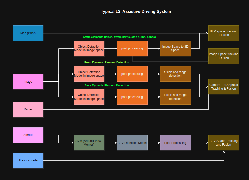
The pipeline diagrams below illustrate common architectures seen in production L2/L2+ systems:
Around View Monitor (AVM / 全景环视系统)
One important pre-processing subsystem is the Around View Monitor (AVM). It provides a seamless top-down surround view by:
- Undistorting fisheye images from multiple surround cameras
- Rectifying each image to a common projection
- Stitching them together into a unified bird’s-eye-view
This is especially valuable for low-speed maneuvers and close-range obstacle detection.
The Typical L2 Perception Stack
In many L2 systems, the map serves as a prior, while the live perception stack combines information from cameras, radar, and sometimes stereo cameras.
A simplified perception chain often looks like this:
Sensors → detection / post-processing → fusion → downstream planning and control
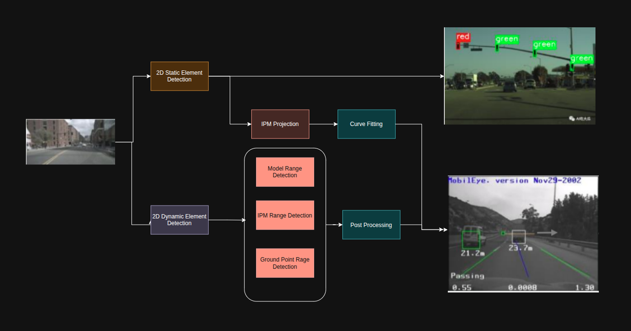
Static Elements
For static scene understanding, the system typically needs to recognize:
- Lane lines
- Traffic lights
- Traffic signs
Most of these start in image space and then need to be lifted into 3D space or transformed into a BEV representation. That transformation is not trivial. For example, lanes may be extracted using image-based detection, inverse perspective mapping (IPM), and curve fitting. Traffic lights and signs may require temporal sequencing across frames to improve stability.
Dynamic Elements
For dynamic objects such as cars and other road users, the system often detects 2D bounding boxes in camera images first, then estimates position and distance through a combination of methods:
- Model-based distance estimation
- IPM-based distance estimation
- Ground-plane-based reasoning
- Radar-assisted localization
- Post-processing and tracking
In many stacks, the front-view perception is camera-dominant, while rear dynamic object detection may be handled separately and sometimes more conservatively, depending on sensor placement and use case.
The practical outputs of such a system may include:
- 2D traffic light and sign detections
- Lane detections
- HD map priors
- Radar-based BEV obstacles
- Camera-based obstacle detections
These are then fused into a more stable world model.
Sensor Fusion Strategies
A central challenge in any multi-sensor system is how to combine information from cameras, LiDAR, and radar. There are two primary paradigms, along with hybrid approaches.
Early Fusion (前融合 / Feature-Level Fusion)
Early fusion aligns LiDAR and camera information as early as possible before feeding it into the model. Common approaches include:
- Projecting point clouds onto the image plane and appending color or image features to each point
- Lifting image features into BEV or 3D space and encoding them alongside point cloud features
The model sees both sensor modalities simultaneously at the intermediate feature stage.
Example: “Attach the camera’s appearance information onto the point cloud first, then jointly decide whether it is a car.”
Key disadvantage: models are usually too big for edge deployment
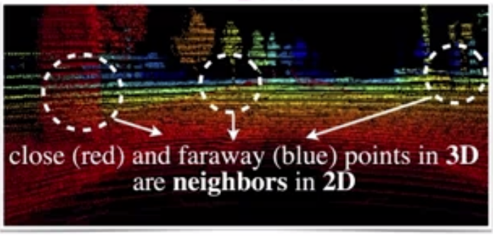
Feature Projection Methods
Feature projection methods such as MMF project 3D features onto 2D. This approach is geometrically lossy: points that are far apart in 3D can appear very close in 2D.
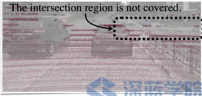
Proposal-Based Methods
Methods like AVOD use proposals to find aligned 2D and 3D features and combine them for detection. These can be semantically lossy when key objects are occluded.
Both feature projection and proposal-based approaches tend to require large models, making them less suitable for deployment on resource-constrained platforms.
Late Fusion (后融合 / Decision-Level Fusion)
Late fusion runs each sensor’s detector independently and merges the results at the output level through:
- Bounding box matching
- Non-maximum suppression (NMS)
- Confidence-weighted merging
- Rule-based or track-level fusion
Example: “The camera says there’s a car here; LiDAR also says there’s a car here — then decide if they refer to the same target and merge.”
A key disadvantage of late fusion is the proliferation of hand-crafted rules, which can become a bottleneck for cross-camera objects and edge cases.
Why Mono3D Is Tempting but Limited
Monocular 3D perception is attractive because it avoids the cost and complexity of extra sensors. But in practice, Mono3D often struggles with accuracy and robustness, especially under long-range, occlusion-heavy, or unusual road conditions.
Data-driven methods for range detection are preferred in principle, but their capabilities are not yet strong enough for full reliance. Representative approaches include:
- FCOS3D — a fully convolutional one-stage monocular 3D object detector with promising results, but requires large datasets and careful tuning
- Mono3D — typically exhibits low accuracy and low robustness in real-world conditions
- Pseudo-LiDAR — converts stereo or mono depth estimates into point clouds, then applies 3D detection; accuracy is often still insufficient to fully replace direct sensing
As a result, many production systems still rely on a mix of geometric priors, hand-engineered post-processing, and deep learning rather than betting entirely on end-to-end monocular 3D.
Today, the mainstream is still a hybrid paradigm: geometry plus deep learning, rather than pure deep learning alone.