Decoder Overview
The overall decoder is looking to achieve the below:
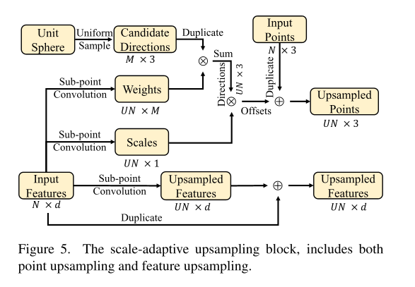
- Icosahedron vertices on a unit sphere become candidate directions — unit vectors pointing from a parent point toward each potential upsampled child.
- Multiple upsampling blocks each independently reference this same set of candidate directions; direction duplication happens across blocks, not within a single block.
- From the sub-point convolution layer, the network learns per-point:
- Weights (convex combination coefficients) over the candidate directions, producing a soft-blended displacement direction per child.
- Scale: a scalar controlling how far along the direction each child is placed (i.e., the displacement magnitude). Scale is learned per-point rather than globally because local point spacing varies across different regions of the cloud.
- Upsampled features: child feature vectors derived from the parent’s input features (e.g., normals, latent descriptors).
- A new upsampled point is placed at:
child_xyz = parent_xyz + direction * weight * scale - A new upsampled feature = upsampled feature + input feature (skip connection, preserving parent information).
The decoder reconstructs a dense point cloud from a compressed latent representation through multiple progressive upsampling stages rather than a single large expansion.
Instead of one large jump:
\[\times 27\]the model applies three sequential steps:
\[\times 3 \;\to\; \times 3 \;\to\; \times 3\]Why progressive upsampling?
-
Numerical stability — a single ×27 expansion requires large coordinate and feature transformations in one step, which can produce unstable gradients and large coordinate jumps. Progressive expansion distributes geometric refinement across smaller, more manageable steps.
-
Staged feature specialization — each block focuses on a different resolution level:
- Block 0: coarse structure recovery
- Block 1: local detail refinement
- Block 2: density adjustment
This is analogous to progressive upsampling in image super-resolution. The overall decoder architecture is:
1
2
3
4
5
6
7
8
9
latent_xyzs
    ↓
Decoder block 0  →  pred_xyzs[0]
    ↓
Decoder block 1  →  pred_xyzs[1]
    ↓
Decoder block 2  →  pred_xyzs[2]
    ↓
Final reconstructed point cloud
Per-block overview
Each decoder layer performs four conceptual steps:
- For each input point, upsample $U$ candidate child points.
- Predict how many upsampled points each input point actually needs.
- Select the appropriate number of candidates.
- Refine the selected points’ coordinates and features.
Step 1 — Candidate Generation
Given inputs:
1
2
xyzs  : (B, 3, N)
feats : (B, C, N)
the model produces $U$ candidates per parent point:
1
2
candidate_xyzs  : (B, 3, N, U)
candidate_feats : (B, C, N, U)
Each candidate child is placed at:
\[\text{child\_xyz} = \text{parent\_xyz} + \text{direction} \times \text{scale}\]- Directions are learned as convex combinations over 43 near-uniform sphere directions (from the icosahedron basis).
- Scales and features are produced by sub-point convolution.
- This is because scale for different regions of the point cloud might be very different.
Step 2 — Predict Upsampling Count
For each parent point the network predicts:
1
upsample_num : (B, N)
This allows variable-density reconstruction — different regions of the point cloud can be upsampled by different amounts. For example:
| Parent point | Children kept |
|---|---|
| Point 0 | 3 |
| Point 1 | 1 |
| Point 2 | 5 |
Total output points: $M = \sum_i \texttt{upsample_num}_i$
Step 3 — Candidate Selection
From the $U$ candidates per parent, the decoder keeps the first upsample_num[i] candidates and flattens across all parents:
1
2
xyzs  : (B, 3, M)
feats : (B, C, M)
For mini-batch training the result is normalized to a fixed target size:
- Too many points ($M >$ target): downsample with FPS.
- Too few points ($M <$ target): pad by randomly repeating existing points.
Step 4 — Refinement
The selected points are refined before being passed to the next stage:
- Coordinate refinement (small residual shifts)
- Feature refinement
- Optional normal reconstruction at the final layer
Output:
1
2
refined_xyzs  : (B, 3, M)
refined_feats : (B, C_out, M)
This becomes the input to the next decoder block.
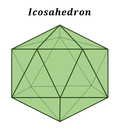
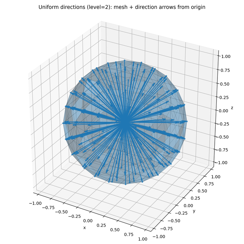
Icosahedron
An icosahedron is a regular solid with 20 triangular faces and 12 vertices. In this project, icosahedron2sphere(level) uses it to generate nearly uniformly distributed directions on a sphere — these serve as candidate upsampling directions when reconstructing point clouds.
A unit icosahedron has all edges of equal length. This holds if and only if its 12 vertices are:
\[(0, \pm 1, \pm \varphi), \quad (\pm 1, \pm \varphi, 0), \quad (\pm \varphi, 0, \pm 1)\]where $\varphi$ is the golden ratio:
\[\varphi = \frac{1 + \sqrt{5}}{2} \approx 1.618\]Using any other value would produce unequal edge lengths.
icosahedron2sphere(level) works as follows:
- Project the icosahedron’s 12 vertices onto a unit sphere.
- If
level > 1, subdivide each triangular face by inserting a new vertex at the midpoint of each edge, then project those new vertices back onto the sphere. - Return the resulting directions, which are nearly uniformly distributed over the sphere.
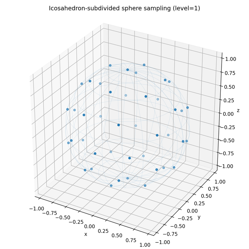
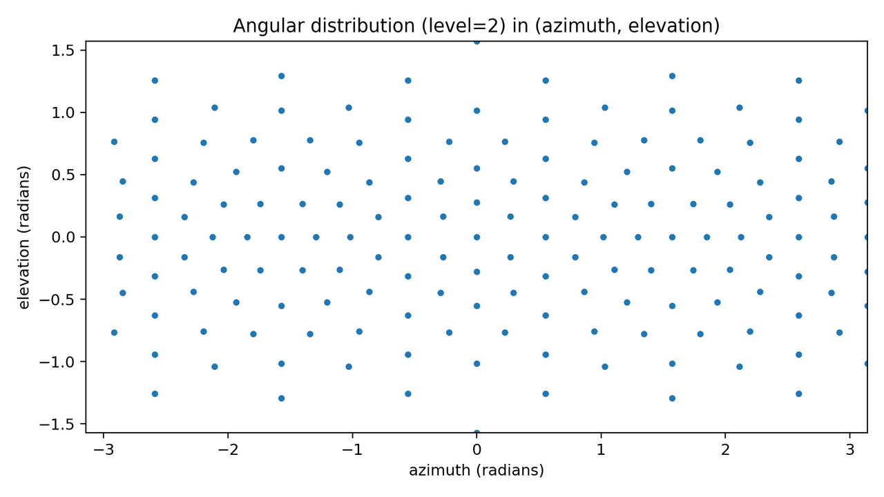
The 12 base vertices are not perfectly uniform, but each subdivision level makes the distribution increasingly uniform. As the return values of this stage, we return
- vertices as 3D coordinates
- triangles’ vertex indices in verticex coordinates above
Below is Level 2 — the midpoints of all edges are added and re-projected:
Sub-Pixel / Sub point Convolution
What is Sub-Pixel Convolution
Given a small low-resolution image (e.g. 4×4), how do you generate a larger high-resolution image (e.g. 8×8)?
-
Vanilla upsampling — bilinear or bicubic interpolation. Fast, but no new fine-grained features are added; the result is a smooth blur.
-
Upsample then convolve — upsample to 8×8, then apply a convolution. Can learn new features, but the convolution runs on the larger image, so it’s expensive.
-
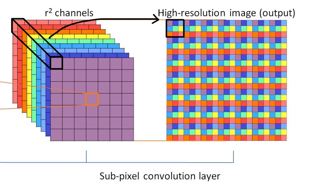
Sub-pixel convolution (convolve then upsample) — apply convolution first on the small image, then rearrange channels into spatial resolution:
Convolution runs on the smaller spatial size, so it is cheaper. The expanded channel dimension (×12) is learned — it is not a simple duplication. Each of the 12 channels is a different learned filter response, and the subsequent pixel-shuffle step interprets those channels as sub-pixel displacements to tile into the higher-resolution output.
Sub-point convolution (the 3-D point cloud analogue) follows the same idea. Each point has a feature vector of dimension $C$. To upsample by factor $r$, convolution first expands the channel dimension to $C \cdot r$, then a point shuffle redistributes those extra channels into $r$ new points — $C$ stays the same:
\[N \times C \;\xrightarrow{\text{conv}}\; N \times (C \cdot r) \;\xrightarrow{\text{point shuffle}}\; (r \cdot N) \times C\]For example, with $N=4$, $C=3$, $r=2$:
\[4 \times 3 \;\xrightarrow{\text{conv}}\; 4 \times 6 \;\xrightarrow{\text{point shuffle}}\; 8 \times 3\]The intermediate $4 \times 6$ representation is learned via convolution, not duplicated — the network packs the information needed to reconstruct 2 new points into those 6 channels.
Pixel Shuffle
The reshape step $4 \times 4 \times 12 \;\to\; 8 \times 8 \times 3$ is called pixel shuffle (or periodic shuffle). It reinterprets the extra channel slots as sub-pixel spatial positions. In a minimal 1D example with upscale factor $r = 2$:
\[[1,\; 2,\; 3,\; 4] \;\xrightarrow{\text{shuffle}}\; \begin{bmatrix} 1 & 2 \\ 3 & 4 \end{bmatrix}\]In 2D, the general form is:
\[H \times W \times (C \cdot r^2) \;\xrightarrow{\text{pixel shuffle}}\; rH \times rW \times C\]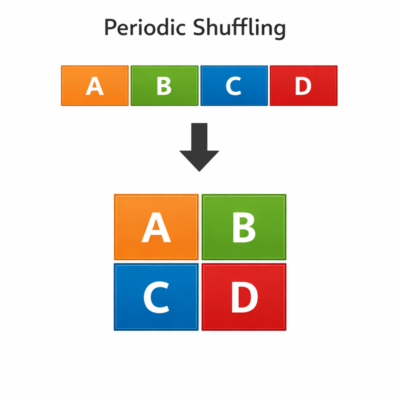
For point cloud compression, why not just copy-then-convolve? The older approach was to first copy (or nearest-neighbour interpolate) the $4 \times 4 \times 3$ feature map 4 times to produce $4 \times 4 \times 12$, then upsample spatially to $8 \times 8 \times 3$ and convolve. The problem is that neighbouring output features all inherited the exact same copied input value, so the network had very little gradient signal to differentiate them — the upsampled points clustered together. Sub-pixel convolution avoids this entirely: the convolution runs on the small feature map and learns genuinely distinct values in each of the $C \cdot r^2$ channels, so every output position starts from a different learned representation.
Sub-Point Convolution
For point clouds the same idea applies along the point dimension instead of spatial H×W. With upsample factor $r$:
\[N \times C \;\xrightarrow{\text{conv}}\; N \times (C \cdot r) \;\xrightarrow{\text{point shuffle}}\; (r \cdot N) \times C\]Upsampling
FeatureUpsampleLayer
feature vector (B, C,N) –> SubpointConv (in_channels = C, out_channels = out_dim upsample_factor) —> (B, out_dim upsample_factor, N, U).
PointCloudUpsampleLayer
1
2
3
4
5
6
7
8
9
10
11
12
13
14
15
16
17
18
19
20
21
22
23
24
25
26
27
28
29
30
31
32
33
34
35
36
37
38
39
40
41
42
43
44
45
46
47
48
49
50
51
52
53
54
55
56
57
58
59
60
61
62
63
64
65
66
67
68
69
70
71
72
73
74
75
76
77
78
79
80
81
82
83
84
85
86
87
88
89
90
91
XyzsUpsampleLayer Forward Pass
═══════════════════════════════════════════════════════════════════════════════

[STATIC] icosahedron2sphere(1) + zero row
  hypothesis: (43, 3) — fixed unit sphere directions on GPU

───────────────────────────────────────────────────────────────────────────────

INPUT
  xyzs  : (B, 3, N)
  feats : (B, C, N)

───────────────────────────────────────────────────────────────────────────────

BRANCH 1 — Weighted Direction For Each Point's Upsampled Point
──────────────────────────────────────────────────────────────

  feats (B, C, N)
    │
    │  SubPointConv — weight_nn
    │    └─ Conv2d(in=C,          out=hidden_dim,  kernel=1)  ─┐  group loop
    │    └─ Conv2d(in=hidden_dim, out=43,          kernel=1)  ─┘  × U groups
    │
    ▼
  weights (B, 43, N, U)
    │
    │  .unsqueeze(2)
    ▼
  weights (B, 43, 1, N, U)
    │
    │  softmax(dim=1)           ← normalise over 43 directions
    ▼
  weights (B, 43, 1, N, U)     — probabilities, sum=1 over dim 1
    │
    │                         hypothesis (43, 3)
    │                           │
    │                           │  repeat("h c -> b h c n u")
    │                           ▼
    │                         hypothesis (B, 43, 3, N, U)
    │
    │  weights * hypothesis    (broadcast over dim=2)
    ▼
  weighted_hypothesis (B, 43, 3, N, U)
    │
    │  sum(dim=1)
    ▼
  directions (B, 3, N, U)
    │
    │  F.normalize(p=2, dim=1)
    ▼
  directions (B, 3, N, U)      — unit vectors

───────────────────────────────────────────────────────────────────────────────

BRANCH 2 — Scale
────────────────

  feats (B, C, N)
    │
    │  SubPointConv — scale_nn
    │    └─ Conv2d(in=C,          out=hidden_dim,  kernel=1)  ─┐  group loop
    │    └─ Conv2d(in=hidden_dim, out=1,           kernel=1)  ─┘  × U groups
    │
    ▼
  scales (B, 1, N, U)

───────────────────────────────────────────────────────────────────────────────

MERGE
─────

  directions (B, 3, N, U)
  scales     (B, 1, N, U)
    │
    │  directions * scales     (broadcast over dim=1)
    ▼
  deltas (B, 3, N, U)
    │
    │                         xyzs (B, 3, N)
    │                           │
    │                           │  repeat("b c n -> b c n u")
    │                           ▼
    │                         xyzs_rep (B, 3, N, U)
    │
    │  xyzs_rep + deltas
    ▼

OUTPUT
  upsampled_xyzs (B, 3, N, U)

═══════════════════════════════════════════════════════════════════════════════
Data Processing
Select First K Points Per Point
For each point $i$ in a batch item, keep only the first upsample_num[b, i] candidates along the upsampling dimension $U$, then concatenate all kept candidates into a flat list of output points.
Example — candidate_xyzs of shape (1, 3, 2, 3) (1 batch, 3D coords, 2 points, 3 candidates each):
| Point | Candidates (u=0,1,2) |
|---|---|
| 0 | (10,0,0), (11,0,0), (12,0,0) |
| 1 | (20,0,0), (21,0,0), (22,0,0) |
candidate_feats of shape (1, 1, 2, 3):
| Point | Feature values (u=0,1,2) |
|---|---|
| 0 | 100, 101, 102 |
| 1 | 200, 201, 202 |
With upsample_num = [[2, 1]] (keep 2 candidates for point 0, 1 for point 1), the output retains points with x-coords [10, 11, 20] — 3 points total.
Multi-Batch Processing
For each batch item bi:
- Call
_select_first_k_per_point(...)to obtain a variable-length selection:sel_xyzs:(1, 3, m)sel_feats:(1, C, m)
where $m = \sum_i \texttt{upsample_num}[bi, i]$.
- Normalize every batch item to the same point count
target_m = int(n * target_rate):- If $m > \texttt{target_m}$: downsample to
target_musing FPS (Farthest Point Sampling). - If $m < \texttt{target_m}$: pad by randomly repeating existing points.
- If $m > \texttt{target_m}$: downsample to
- Concatenate across the batch dimension to produce:
xyzs_out:(B, 3, target_m)feats_out:(B, C, target_m)