Robot Navigation ESDF

ESDF

There are two common approaches for incremental ESDF construction in robotics: Voxblox and Fiesta.

Here we describe the core idea behind the 1D Euclidean Distance Transform (EDT) used in Fast Planner, based on: Felzenszwalb & Huttenlocher, “Distance Transforms of Sampled Functions”

1D Euclidean Distance Transform

Consider a 1D voxel grid with indices

\[p \in [0, n-1]\]

Distance is euclidean distance, not Manhattan Distance.
f(p) = 0 at obstacle locations, otherwise it’s $\inf$

Assume obstacles are in $Q$, then the distance field value at index $p$ is to find the minimum distance among all obstacles Q:

\[D(p) = min_{Q} ((p - q) ^ 2 + f(q)\]

The goal is equivalent to finding the lower Envelope of the quadratic functions

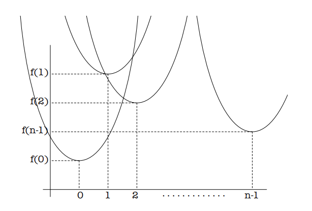
It’s easy to find the intersection between two such parabolas:

\[(p-q_1)^2 + f(q_1) - ((p-q_2)^2 + f(q_2)) \\ \Rightarrow \\ p = \frac{f(q_1) + q_1^2 - f(q_2) - q_2^2}{2(q_1 - q_2)}\]

Then, voxels in to the left and the right of the intersections will get distance field values from the corresponding parabola.

Now we are going to have one very important property:

Since all parabolas have the same quadratic terms, any two parabolas intersect at most once despite of their relative positions

This property is what makes the algorithm linear time.

So now, we can start finding distance value from the leftmost 1D voxel.

# f is 1D array. Distance from x to parabola p is (x-p)^2 + f[p]
# obstacles at m will have f[m] = 0. Free cell n has f[n] = INF
def distance_tf_1d(f):

 # 
 n = f.shape[0] # number of voxels 
 v = np.zeros(n, dtype=np.int32)  # The x coordinate of the lowest point of each parabola, the "valleys"
 z = np.zeros(n + 1, dtype=np.float64) # left boundaries of all parabolas   
 d = np.zeros(n, dtype=np.float64) # final distance field  

 k = 0 
 v[0] = 0
 z[0] = - INF
 z[1] = + INF
 
 
 # intersection between two parabolas
 def intersect(q1, q2):
  return ((f[q1] + q1*q1) - (f[q2] + q2*q2)) / (2.0*(q1 - q2))

 for q in range(0,n):
  p = intersect(v[k], q)
  # q will only be larger than v[k]. If the intersection is to the LEFT of the k-th parabola's break point, that means q-th parabola is below k-th parabola for that entire range. In that case, we will replace the k-th parabola
  while p <= z[k]:
   k -= 1
   p = intersect(v[k], q)
  k += 1
  v[k] = q
  z[k] = p
  z[k+1] = INF

 # walk along x axis from 0 to n
 # you now have z[k+1] defines the break points of the envelope
 # v[k] is the index of parabolas at k.
 k = 0
 for q in range(n):
  while z[k+1] < q:
   k += 1
  p = v[k]
  d[q] = (q - p) * (q - p) + f[p]
 return d

Extending to N-D

The beauty of this algorithm is that for N-dimensions, you can apply this algorithm independently.

Assume that we have a 2D map. First, apply 1D Distance Transform along each row (x axis). Then, for the rows with obstacles, each cell has a distance value to their nearest row obstacle. $D(x,y) = min ((x - i) ^ 2 + F(i,y))$

Now, apply distance transform along each column. $D(x,y) = min_j((y - j)^2 + G(x,j) )$ You scan through voxels along this column, which already provide distance values there. Still clear as mud? Let’s walk through an example:

In this grid, let the only obstacle be at (2,1).

(0,2) (1,2) (2,2)  
(0,1) (1,1) (2,1)  
(0,0) (1,0) (2,0)

So We want squared Euclidean distance:

\[D(x,y) = (x - 2)^2 + (y-1)^2\]

Step 0 — Initial grid F

We define:

F = 0 at obstacle
F = INF elsewhere

y=2:  INF  INF  INF  
y=1:  INF  INF   0  
y=0:  INF  INF  INF

Step 1 — 1D EDT along x (row by row)

We now compute for each row:

\[D(x,y) = min ((x - i) ^ 2 + F(i,y))\]

y=2:  INF  INF  INF  
y=1:    4    1    0  
y=0:  INF  INF  INF

Step 2 — 1D EDT along y (column by column)

$D(x,y) = (x - 2)^2 + (y-1)^2$ Column 1 is

y=2: INF  
y=1: 4  
y=0: INF

For y=0, x=1,

\[D(0,y) = (y-1)^2 + 4 = 5\]

Then you can see that 4 already the x-axis distance of the column to the obstacle. Adding $(y-1)^2$ directly gives the distance! So the final values are:

y=2:  5   2   1  
y=1:  4   1   0  
y=0:  5   2   1

Which is exactly $D(x,y) = (x - 2)^2 + (y-1)^2$

What Is a Signed Distance Field?

A signed distance field returns:

\[\phi(x) = \begin{cases} +\text{distance to the nearest obstacle}, & \text{if } x \text{ is in free space}, \\[6pt] 0, & \text{if } x \text{ lies on the obstacle surface}, \\[6pt] -\text{penetration depth}, & \text{if } x \text{ is inside an obstacle}. \end{cases}\]

Why We Need a Signed Distance Field (Negative Distances Matter)

Many modern planners like Fast-Planner do not rely on graph search (A*, RRT, etc.).
Instead, they use trajectory optimization. They represent a trajectory as a smooth function:

$x(t)$ and minimize a cost of the form:

\[J = J_{smooth} + \lambda J_{collision}\]

$J_{smooth}$: encourages smooth motion, like minisnap, minijerk, etc.
$J_{collision}$: keeps trajectory away from obstacles. This depends on the signed distance field:

\[\phi(x) = \text{signed dist to obstacle}\]

Consider a single point on the trajectory: $x_k$. Suppose it is slightly inside a wall:

$\phi(x_k) < 0$ We define a collision penalty:

$J_{collision}(x_k) = \frac{1}{2} max(0, d_{safe} - \phi(x_k))^2$ The optimizer moves the trajectory by following the gradient of the cost.

\[\nabla J = -(d_{safe} - \phi(x_k)) \nabla \phi(x_k)\]

$\nabla \phi(x)$ is the gradient of the signed distance field. It points outward from the obstacle, and has magnitude $\approx 1$ near surface. If you are instead the wall, it will point outward too. In gradient descent update:

$x_k = x_k - \alpha \nabla J = x_k + \alpha(d_{safe} - \phi (x_k)) \nabla \phi(x_k)$ $x_k$ will be pushed outward, too. Therefore, if we do NOT use negative distances within obstacles, $\phi(x) = 0$, so $x_k$ gets stuck and won’t be pushed out

References

[1] Zhihu