Robotics - [3D SLAM - 2] Lidar Odometry - Rico贾若童的博客

Direct Lidar Odometry

When given two scans, a direct NDT method means no features are extracted. The two scans would directly go through NDT for finding their relative poses. The workflow is as follows

scan -> NDT ---pose_estimate---> Is_Keyframe? ---yes---> Add_Frame

NDT Odometry

I’m implementing a robust 3D NDT-based Odometry system, and it’s been a rewarding challenge! Here’s a quick breakdown of how it works, plus some lessons learned and visual results.

NDT Registration:
1. Build hash map that represents voxels from all point clouds of the current submap [INEFFICIENT]
2. Calculate the mean and variance of the voxels
3. Update motion_model = last_pose.inverse() * pose
  - This can be used as the pose initialization
Keyframe Detection:
1. 📐 Trigger a new keyframe if the pose has shifted significantly in angle or translation
Frame Integration Pipeline Scan → NDT Alignment → Keyframe Check → (If Yes) Add to Map

Here, you can check out my implementation

NDT LiDAR Odometry Visualization Without Skipping Frames

💡 Key Takeaways

✅ Always voxel-filter input scans in pre-processing — it massively reduces noise and speeds things up.
📌 Only keyframes are used to build the target map. Non-keyframes still contribute to visualization but don’t clutter the optimization.
🧩 For sparse data, you have two options for Nearby6 voxel association:
- 🔺 Aggregate all voxel errors (can explode to 10⁷+ for large clouds!)
- ✅ Use only the best voxel — leads to more stable optimization
🐛 PCL versions matter:
- PCL 1.12 has a spinOnce() bug. PCL 1.13 is stable but slow
- PCL 1.14 is much better

Incrememental NDT Odometry

The high level workflow of Incremental NDT is the same as the non-incremental one:

scan -> NDT ---pose_estimate---> Is_Keyframe? ---yes---> Add_Frame

Incremental NDT Visualization Without Skipping Frames

The main difference, however, is in add_frame:

Given two point clouds: source and target, we can voxelize them.
For the same voxel location in source and target:
1. Count the number of points in the voxel of source and target: m, n
2. We can calculate mean and variances of them: $\mu_a$, $\mu_b$, $\Sigma_a$,$\Sigma_b$
3. Now we want to add the source cloud to the target. We can update the target point cloud’s new mean directly:
  \[\begin{gather*} \begin{aligned} & \mu = \frac{x_1 + ...x_m + y_1 + ... y_m}{m + n} = \frac{m \mu_a + n \mu_b}{m + n} \end{aligned} \end{gather*}\]
4. For the target’s new variance (ignoring Bessel correction):
\[\begin{gather*} \begin{aligned} & \Sigma = \frac{1}{m+n} (\sum_i (x_i - \mu)(x_i - \mu)^T + (y_i - \mu)(y_i - \mu)^T) \\ & \sum_i (x_i - \mu)(x_i - \mu)^T = \sum_i (x_i - \mu_a + (\mu_a - \mu))(x_i - \mu_a + (\mu_a - \mu))^T \\ & = \sum_i [(x_i - \mu)(x_i - \mu)^T + (x_i - \mu_a)(\mu_a - \mu)^T + (\mu_a - \mu)(x_i - \mu_a)^T + (\mu_a - \mu)(\mu_a - \mu)^T] \\ & \text{one can see that} \sum_i (x_i - \mu_a)(\mu_a - \mu)^T = 0 = \sum_i (\mu_a - \mu)(x_i - \mu_a)^T \\ & \Rightarrow \sum_i (x_i - \mu)(x_i - \mu)^T = m \Sigma_a \\ & \text{So ultimately:} \\ & \Sigma = \frac{1}{m+n}[m (\Sigma_a + (\mu_a - \mu)(\mu_a - \mu)^T) + n(\Sigma_b + (\mu_b - \mu)(\mu_b - \mu)^T)] \end{aligned} \end{gather*}\]
Also, if we want to discard voxels if there have been too many old ones, we can implement an Least-Recently-Used (LRU) cache of voxels.

If there are too many points in a specific voxels, we can choose not to update it anymore.

Summary of Vanilla and Incremental NDT Odometry

Similarities:

We don’t store points into point cloud permanently. We just store voxels and their stats

How do we update voxels?

NDT3D needs a grid_: unordered_map<key, idx>. This means:
1. We need to reconstruct the grid cells from scratch.
2. We need keyframes which allows us to selectively add ponitclouds
NDT3D_inc needs an LRU cache: std::list<data>, unordered_map<itr>. We don’t need to generate grid cell

Indirect Lidar Odometry

Indirect Lidar Odomety is to select “feature points” that can be used for matching. There are 2 types: planar and edge feature points. This was inspired by LOAM (lidar-odometry-and-mapping), and is adopted by subsequent versions (LeGO-LOAM, ALOAM, FLOAM). Indirect Lidar Odometry is the foundation of LIO as well. Common features include: PFH, FPFH, machine-learned-features. Point Cloud Features can be used for database indexing, comparison, compression.

LeGO-LOAM uses distance image to extract ground plane, edge and planar points; mulls uses PCA to extract plane, vertical, cylindircal, horizontal features.

After feature detection, we can do scan-matching using ICP or NDT

Some characteristics of 3D Lidar points are:

They are not as dense as the RGB-D point cloud. Instead they have clear line characteristics.
Should be lightweight. Not much CPU/GPU is used
- So people in industry LO systems use simple features instead of complex ones, learned by machine learning systems.
Computation should not be split - some on CPU, some on GPU.

Edge points along their vertical direction can be used for point-line ICP; planar points can be used for point-plaine ICP.

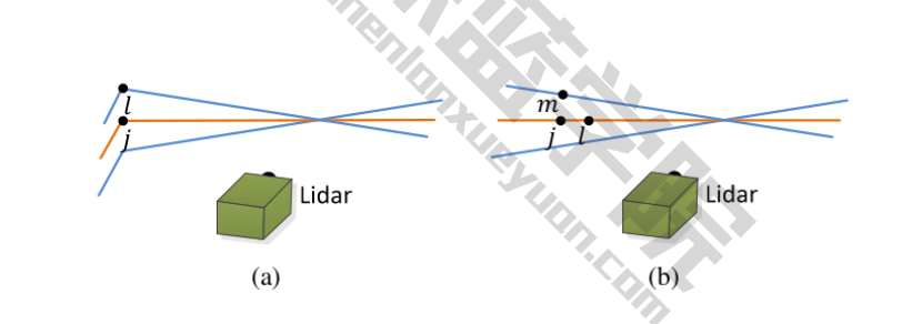
LOAM-Like Feature Extraction

Feature-based LO have better general usability than point-point ICP or point-plane ICP. In the autonomous vehicle industry, LOAM, LeGO-LOAM, ALOAM, FLOAM are common solutions. They are the foundation of many LIO systems, but due to the complexity of LOAM’s code, here we have a simplified version.

For any LOAM system, we mostly care about “what features shall we extract”? Common features include PFH, FPFH, and many other deeply-learned features. In the industry, people currently use simple, hand-crafted features. This is because we don’t want to take up too much CPU/GPU resources.

A simple hand-crafted feature extraction method is based on LiDAR scan lines. Each line has a timestamp, which makes our nearest-neighbor-search much easier. In LOAM, we extract planar and edge points. Such a concept can be used in 2D Scan-Matching as well. In 3D, LeGO-LOAM extracts ground, planar, and edge points using distance image? MULLS (Multi‐metric Linear Least‐Square, 2021) classfies points into semantic/geometric groups (ground, facade, pillars, beams, etc.) via dual‐threshold ground filtering and PCA. Of course, RGBD SLAM / Solid-State LiDAR SLAM methods do not have scan lines. So we cannot use such methods here.

This line of thoughts can be applied in 2D lidars as well.

- extract_feature
    1. For each point in scan[5, size-5)
        1. calculate curvature:
            dx = sum(nearest 10 neighbors) - 10 * self.x
            curvature = dx^2 + dy^2 + dz^2
    2. seglength = total_points / 6;  for(i = 0; i < 6; i++)
        seg_start = i * seg_length
        seg_end = (i+1) * seg_length
        extract_feature_from_segment(seg_start, seg_end)

- extract_feature_from_segment:
    1. sort points by curvature, (from low to high)
    2. start from the end (largest curvature):
        1. Reject curvatures less than 0.1
        2. Add point to edge_list, and the ignored_list
        3. Break if edge points have exceed a threshold
        4. Check the left 5 neighbors. 
            1. Calculate its ruggedness of [k-1], [k]. 
            2. If ruggedness < threshold, add to ignored_list
        5. Repeat for the right 5 neghbours
    3. loop over the curvature list
        1. If the point is not in the ignored list, add to the surface_list

Why Segment Scans?

We evaluate a point’s “ruggedness” (local curvature) against its neighbors to choose edge and planar features. Without segmentation, high-curvature areas would dominate, leaving other directions underrepresented. By dividing each scan line into fixed angular sectors (e.g., six), we ensure a balanced quota of features from every part of the scan, yielding uniform spatial coverage.
Handling degeneracy along a wall When the sensor travels parallel to a long, flat surface, all strong edges lie in roughly the same direction—this can make the Hessian in our optimizer rank-deficient. Segmentation forces us to pick features from multiple sectors (including those opposite the wall), which restores geometric diversity and prevents loss of observability.

Differences From The LOAM Paper

In the original paper:

First, points are time-warped to the beginning of the scan using either a linear “twist” model or IMU interpolation before curvature is computed (ScanRegistration §3.1)
For each scan line/beam, divide the point cloud into six sectors (each takes 1/6 of start-end index diff), and extract sharp (corner) and flat (plane/surface) features as follows.
- In each sector, sort cloud index according to curvature. The top 2 largest curvature points (if points are not selected and curvature > 0.1) are marked as sharp, the top 20 largest curvature points are marked as less sharp (including the top 2 sharp points), the top 4 smallest curvature points (with additional condition curvature < 0.1) are marked as flat, and all the rest points plus the top 4 flat points will be down sampled and marked as less flat.
  - In real life, the classification of sharpness could indeed increase robustness in some scenarios
  - LeGO-LOAM, MULLS LOAM have different extractions, but the scan matching processes are the same (ICP)
- After each feature extraction, there will be a non-maximum suppression step to mark neighbor 10 points (+-5) to be already selected (marking will stop at points that are 0.05 squared distance away from currently picked point), so that they will not be picked in the next iteration for feature extraction.
- A downsample operation (of leaf size 0.2m) is applied to each scan of less flat points, and then all downsampled scans are combined together (into one point cloud) to be published to odometry.
For example for VLP-16 LiDAR, there could be 384 flat feature points and 192 sharp feature points extracted in a point cloud frame (if all meet the 0.1 curvature threshold).
KD Tree is used for fast indexing

However, the original paper has some drawbacks too:

Most numbers are “magic constants” set in launch file or hard coded

Take-Aways From A Hands-On LOAM-Like Odometer

Voxel filtering is still essential, but please do that when adding keyframes. Otherwise, there would be fewer edge & planar features.
Using last_pose and second_last_pose is better for motion modelling than last keyframe pose, and second last keyframe poses.
LOAM， A-LOAM, LeGO-LOAM, LIO-SAM assume the existence of scan line ordering in each point cloud. If such ordering does not exist, e.g., in Hesai AT-128 / Livox mid-360, one should use voxel-based method like NDT / GICP.

Robotics - [3D SLAM - 2] Lidar Odometry

Direct Lidar Odometry, NDT, Incremental NDT, Indirect Lidar Odometry