Robotics - [3D SLAM - 1] Scan Matching - Rico贾若童的博客

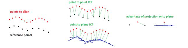
Point-Point ICP

If we write out our state vector as [theta, translation], the pseudo code for point-point ICP is:

pt_pt_icp(pose_estimate, source_scan, target_scan):
    build_kd_tree(target_scan)
    for n in ITERATION_NUM:
        for pt in source_scan:
            pt_map = pose_estimate * pt
            pt_map_match = kd_tree_nearest_neighbor_search(pt_map)
            errors[pt] = pt_map_match - pt_map
            jacobians[pt] = [pose_estimate.rotation() * hat(pt_map), -Identity(3)]
        total_residual = errors* errors
        H = sum(jacobians.transpose() * jacobians)
        b = sum(-jacobians.transpose() * errors)
        dx = H.inverse() * b
       pose_estimate += dx;
        if get_total_error() -> constant:
            return

Note that in Point-Point ICP, for scan matched point (in map frame) p_i and its matched point q_i, if pose estimate is decomposed into [R, t], we set:

\[\begin{gather*} \begin{aligned} & e = q_i - Rp_i - t \\ & \frac{\partial e}{\partial R} = R[p_i]^\land, \frac{\partial e}{\partial t} = -I \end{aligned} \end{gather*}\]

Notes

Iterative Method is not a must. Unlike the above point association -> pose estimate -> … iteration, recent scan matching methods solve point association and pose estimate together. TODO?
- Iterative methods are relatively simpler, though. It works as long as the cost landscape is decreasing from the current estimate to the global minimum.

Point-Plane ICP

If we write out our state vector as [theta, translation], the pseudo code for point-plane ICP is:

pt_plane_icp(pose_estimate, source_scan, target_scan):
    build_kd_tree(target_scan)
    for n in ITERATION_NUM:
        for pt in source_scan:
            pt_map = pose_estimate * pt
            N_pt_map_matches = kd_tree_nearest_neighbor_search(N, pt_map)
            plane_coeffs = fit_plane(N_pt_map_matches)
            errors[pt] = signed_distance_to_plane(plane_coeffs, pt_map)
            jacobians[pt] = get_jacbian(plane_coeffs, pt_map)
        total_residual = errors* errors
        H = sum(jacobians.transpose() * jacobians)
        b = sum(-jacobians * errors)
        dx = H.inverse() * b
       pose_estimate += dx;
        if get_total_error() -> constant:
            return

The Point-Plane ICP is different from Point-Point ICP in:

We are trying to fit a plane instead of using point-point match
In real life, we need a distance threshold for filtering out distance outliers.

Also note that:

A plane is $n^T x + d = 0$. The plane coefficient we get are $n, d$
The signed distance between a point and a plane is:

\[\begin{gather*} \begin{aligned} & e_i = n^T(R q_i + t) + d \end{aligned} \end{gather*}\]

The jacobian of error is:

\[\begin{gather*} \begin{aligned} & \frac{\partial e_i}{\partial R} = -n^T R q^\land \\ & \frac{\partial e_i}{\partial t} = n^T \end{aligned} \end{gather*}\]

Point-Line ICP

The point-line ICP is mostly similar to the point-plane ICP, except that we need to adjust the error and Jacobians.

A line is:

\[\begin{gather*} \begin{aligned} & d \vec{r} + p_0 \end{aligned} \end{gather*}\]

We choose the error as the signed distance between a point and it is :

\[\begin{gather*} \begin{aligned} & e = \vec{r} \times (R p_t + t - p_0) \\ & = \vec{r} ^ \land (R p_t + t - p_0) \end{aligned} \end{gather*}\]

The jacobian is:

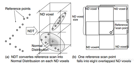
\[\begin{gather*} \begin{aligned} & \frac{\partial e}{\partial R} = - \vec{r} ^\land R p_t^{\land} \\ & \frac{\partial e}{\partial t} = \vec{r} ^\land \end{aligned} \end{gather*}\]

NDT (Normal Distribution Transform)

Voxelization. Partition the target point cloud into voxels. For each voxel, compute:
- Mean: $\mu$
- Covariance matrix: $\Sigma$
Point-to-Distribution Association (for each source point). For each point $p_t$ in the source scan:
1. Transform to map frame using current pose estimate: $p_t = Rp_t + t$
2. Voxle Lookup. Find the voxel containing $pt$ in the target map. Retrieve $\mu$ and $\Sigma$ of that voxel.
3. Error and cost function:
  1. Assuming correct alignment, the transformed point should follow the distribution of the voxel:
    \[e_i = Rp_t + t - \mu \\ \text{error}_i = e_i^T \Sigma^{-1} e_i\]
  2. Here, $\Sigma$ is the covariance matrix of the voxel. $\Sigma^{-1}$ is the information matrix, and because we are getting its inverse, in practice, we want to add a small value to it $\Sigma + 10^{-3}I$
  3. Jacobian update:
    \[\begin{gather*} \begin{aligned} \frac{\partial e_i}{\partial R} = -Rp_t^\land \\ \frac{\partial e_i}{\partial t} = I \end{aligned} \end{gather*}\]
4. We also consider neighbor cells as well, because the point might actually belong to one of them. So we repeat step 3 for those voxels.
Maximum Likelihood Estimate (MLE):

$\begin{gather*} \begin{aligned} & (R,t) = \text{argmin}_{R,t} [\sum e_i^t \Sigma^{-1} e_i] \\ & = \text{argmax}_{R,t} [\sum log(P(R q_i + t))] \end{aligned} \end{gather*}$
- $H = \sum_i J_i^T info J_i$
- $b = -\sum_i J_i^T info e_i$
- $\Chi^2 = \sum_i e_i^T info e_i$
- $dx = H^{-1} b$

When the point cloud is sparse, we need to consider neighbor voxels. While it’s dense, 1 voxel is enough for matching.

Advantages and Weaknesses:

NDT is very concise, and it does not need to consider plane, or line like ICP. It has become a widely-used baseline scan matching method.
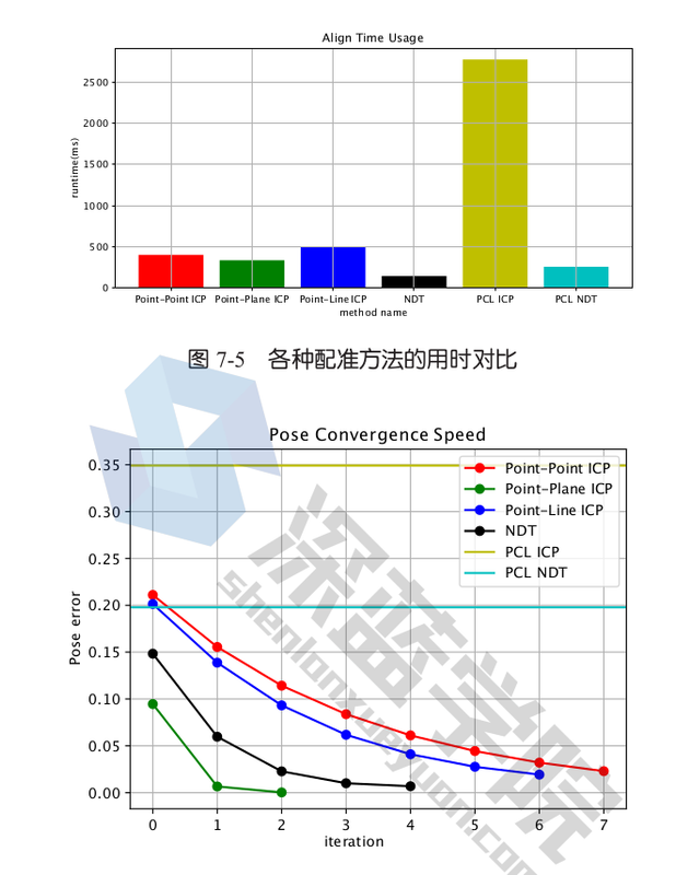
In general, it’s much faster than ICP methods, and its performance is a little worse than pt-plane ICP, but better than pt-pt ICP and is similar to pt-line ICP.
However, like many other scan-matching method, NDT is prone to bad pose intialization. Also, voxel size could be a sensitive parameter.

This is more similar to the 2D version of NDT [2], and it different from the original paper [1]. But the underlying core is the same: in 2009, SE(3) manifold optimization was not popular, therefore the original paper used sin and cos to represent the derivative of the cost function. In reality, modifications / simplifications like this are common.

Another consideration is that we add a small positive value to the covariance matrix, because we need to get its inverse. When points happen to be on a line or a plane, elements on its least principal vectors will become zero.

Why NDT Works

We have points in the target cloud x1, x2...xi and source cloud x1', x2' ... xi'. The goal is to find the transform T such that $x1 \approx T x1’$ …

The mean and covarance matrix of the target cloud are $\mu_t$, $\Sigma_t$

The main idea of NDT is “if the true transform T* is found, the point distrbution of the source and the target clouds should match at each voxel.” - We are actually turning the target cloud into a statistical field - The main idea can also be phrased as “How probable is my source cloud if I move it by T?”

One necessary condition of the aforementioned optimization procedure to implement the main idea is:

“Probability Density Function value (PDF) of the source cloud w.r.t the target cloud is maximized when the ‘true transform’ T* is applied:”

\[\begin{gather*} \begin{aligned} & \prod_I f((T^{*})^{-1} x_i') \\ & \text{where f(x) is the pdf of the target cloud points} \\ & f(x) = \frac{1}{(2\pi)^{d/2} |\Sigma_t|^{1/2}} \exp\left( -\frac{1}{2} (\mathbf{x} - \boldsymbol{\mu}_t)^\top \Sigma_t^{-1} (\mathbf{x} - \boldsymbol{\mu}_t) \right) \end{aligned} \end{gather*}\]

Here is the proof:

The product form above really is the joint PDF of all source cloud points w.r.t the target cloud. It’s equivalent to summing the log of it (a.k.a Mahalanobis Distance):

\[\begin{gather*} \begin{aligned} & \sum_{i=1}^N (\mathbf{x}_i - \boldsymbol{\mu}_t)^\top \Sigma_t^{-1} (\mathbf{x}_i - \boldsymbol{\mu}_t) := ln(f(X)) \end{aligned} \end{gather*}\]

Given a candidate pose T, the expected log-likelihood of all the source cloud points are

\[\begin{gather*} \begin{aligned} & E_T[ln(f(T^{-1}X'))] = \sum_N E_T[ln(f((T^{*})^{-1} x_1'))] + E_T[(T^{*})^{-1} ln(f(x_2'))] + ... \end{aligned} \end{gather*}\]

$x_1’$, $x_2’$ are samples from the source cloud, and they are independent from each other. So they can be thought of as samples drawn from the source cloud distribution $X’$

\[\begin{gather*} \begin{aligned} & E_T[ln(f(T^{-1} x_1'))] = E_T[ln(f(T^{-1} X'))] \end{aligned} \end{gather*}\]

To calculate the expected log-likelihood, we have a refresher: the expectation of a function $g(X)$ is:

\[\begin{gather*} \begin{aligned} & E[g(x)] = \int g(x) p_X(x) dx \end{aligned} \end{gather*}\]

So for a point in source cloud $X’$, we need to find the true corresponding pdf value of $ln(f(x_i’))$. Following the true transform, each point $x_i’$ is mapped to target point $x_{i} = (T^*)^{-1} x_{i}’$. But under the candidate pose T, they are mapoped to $x_{iT} = T^{-1} x_{i}’$. So the true corresponding pdf value of $ln(f(T^{-1}f(\mathbf{x}_i’)))$ should be:

\[\begin{gather*} \begin{aligned} & p_X(x) = f\left((T^*)^{-1} \mathbf{x}_i'\right) \\ & \Rightarrow \mathbb{E}_T\left[\ln(f(\mathbf{X}'))\right] = \mathbb{E}_T\left[\ln\left(f(T^{-1} \mathbf{x}_i')\right)\right] = \int f\left((T^*)^{-1} \mathbf{x}_i'\right) \ln\left(T^{-1}f(\mathbf{x}_i')\right) \, d\mathbf{x} \\ & = f_{T^*}(\mathbf{x}_i) \ln\left( f_T(\mathbf{x}_i) \right) \end{aligned} \end{gather*}\]

This form happens to be conveniently represented as

\[\begin{gather*} \begin{aligned} \int f((T^*)^{-1} \mathbf{x}_i') \ln(f(\mathbf{x}_i')) \, d\mathbf{x} &= \mathbb{E}_{T^*}[\ln(f(\mathbf{X}'))] - \int f_{T^*}(\mathbf{x}_i) \ln\left( \frac{f_{T^*}(\mathbf{x}_i)}{f_T(\mathbf{x}_i)} \right) \, d\mathbf{x}_i \\ &= \mathbb{E}_{T^*}[\ln(f(\mathbf{X}'))] - D_{\mathrm{KL}}(f_{T^*} \,\|\, f_T) \\ &\text{(This is the KL divergence)} \end{aligned} \end{gather*}\]

And KL Divergence cannot be negative. See here for proof. So, now we have completed the proof

Then, the scan matching problem becomes finding the T such that the total Mahalanobis distance of source points w.r.t the target cloud is minimized.

Comparison

PCL is slower because we are using spatial hashing to find neighboring cells. PCL NDT uses a KD tree for that. A Kd-tree is built over the centroids of those cells

References

[1] M. Magnusson, The three-dimensional normal-distributions transform: an efficient representation for registra- tion, surface analysis, and loop detection. PhD thesis, Örebro universitet, 2009.

[2] P. Biber and W. Straßer, “The normal distributions transform: A new approach to laser scan matching,” in Proceedings 2003 IEEE/RSJ International Conference on Intelligent Robots and Systems (IROS 2003)(Cat. No. 03CH37453), vol. 3, pp. 2743–2748, IEEE, 2003.

Robotics - [3D SLAM - 1] Scan Matching

3D Point-Point ICP, 3D Point-Plane ICP, NDT