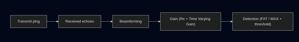
Sonar Imaging Pipeline
Here is a nice introduction to the concept of beam-forming
Beam Forming
If you have multiple attenae, say each attena is attached to a fixed delay, then the waves from the attenae will have different phases. If these delays are fine-tuned, these waves will amplify each other at a certain angle, and will attentuate at other angles
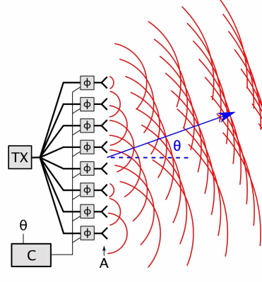
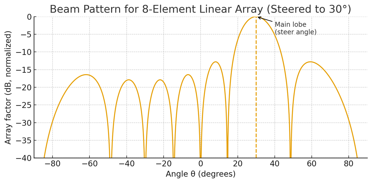
The magnitudes of the waveform at each angle is illustrated as follows
1
2
3
4
5
6
7
8
9
10
11
12
13
14
15
16
17
18
19
c = 1500.0
f = 30000
wave_length = c / f
wave_number = 2 * np.pi / wave_length
num_elements = 8
element_spacing = wave_length / 2
steer_angle = 30  # degrees

def get_array_factor(theta_arr, intended_steer_angle):
    theta_rad = np.deg2rad(theta_arr)
    steer_rad = np.deg2rad(intended_steer_angle)
    n = np.arange(num_elements).reshape(-1, 1)
    phase = (np.sin(theta_rad) - np.sin(steer_rad)) * wave_number * element_spacing * n
    array_factor_magnitudes = np.abs(np.sum(np.exp(1j * phase), axis=0))
    return array_factor_magnitudes / np.max(array_factor_magnitudes)

theta_arr = np.linspace(-90, 90, 721)
array_factors = get_array_factor(theta_arr, steer_angle)
array_factors_db = 20 * np.log10(array_factors + 1e-12)
Amplification
After we’ve formed the beams, we wait for echoes to arrive and then run them through the receive chain.
Rx gain is applied in the analog front end at the hydrophone’s amplifier. It boosts all received signals before digitization so they sit in a usable range for the ADC and later processing, instead of being buried in quantization noise.
TVG (Time Varying Gain) is a range-dependent gain applied as a function of time. As sound travels farther, its energy spreads out and is absorbed by the water, so distant echoes are much weaker than near ones. TVG compensates for this by applying more gain to later (farther) samples and less gain to earlier (closer) samples. The result is that targets at different ranges become more comparable in amplitude, making a single detection threshold practical across the whole water column.
Detection and Synchronization
With beamforming and amplification done, we can finally decide whether and where each beam “sees” a target.
For each beam at angle θ, we have a time series E(θ,t) representing the signal strength (often expressed in dB) as a function of time t, which maps to range. Based on this time series, we can choose different detection strategies:
- FAT (first above threshold): detect the first return that’s above a certain noise threshold
- MAX: detect the strongest return regardless of when it arrives
Aligning pings and range calculation depends heavily on timing. For synchronization, we use Chrony, a highly accurate Network Time Protocol.