Computer Vision - Uzzle Solver

Step 1 Preprocessing TODO

1. Convert the camera frame from color → grayscale

2. Apply a Gaussian blur to reduce noise and stabilize edges

3. Dilate edges so boundaries are thicker and more connected

Step 2 - FindContour

A contour is a sequence of points that lie along the boundary of a connected region (object) in an image. In OpenCV, contours are typically extracted from a binary image, where pixels are split into foreground and background.

• For better accuracy, use binary images. So before finding contours, apply threshold or canny edge detection
• The algorithm requires background to be white and borders to be black.
• cv2.RETR_TREE is contour retrieval mode
• CHAIN_APPROX_SIMPLE is the contour approximation method

1
im2, contours, hierarchy = cv2.findContours(thresh, cv2.RETR_TREE, cv2.CHAIN_APPROX_SIMPLE)

• Args
  • Retrieval mode (cv2.RETR_TREE, cv2.RETR_EXTERNAL, …)
    • RETR_TREE: returns all contours and reconstructs full parent/child hierarchy (outer contours + holes).
    • RETR_EXTERNAL: returns only the outermost contours (often simplest).
  • Approximation method (cv2.CHAIN_APPROX_SIMPLE, cv2.CHAIN_APPROX_NONE)
    • CHAIN_APPROX_SIMPLE: compresses horizontal/vertical segments (fewer points).
    • CHAIN_APPROX_NONE: keeps every boundary pixel (more points).
• Returns:
  • contours is a list[np.array(x, y), ...] of boundary points in the image. Shape is typically (N, 1, 2) and points are (x, y) (x = column, y = row).
  • hierarchy: array describing contour nesting (parent/child relationships), useful for holes.

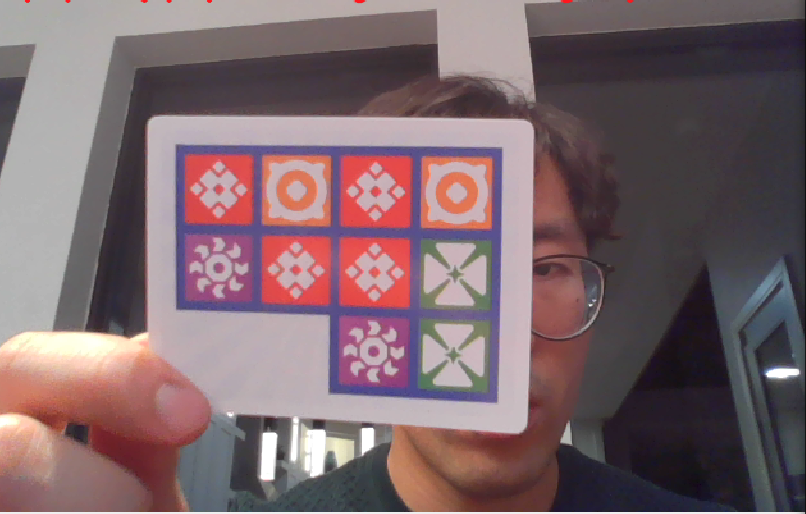
1) Input image (grayscale)

The raw image before any preprocessing. At this stage, contours are not well-defined because foreground and background are not separated yet.

2) Thresholded binary image

We convert the image into a binary representation so that the object pixels become one value (e.g., 255) and the background becomes 0 (or vice versa). Contour algorithms usually assume a clean binary separation.

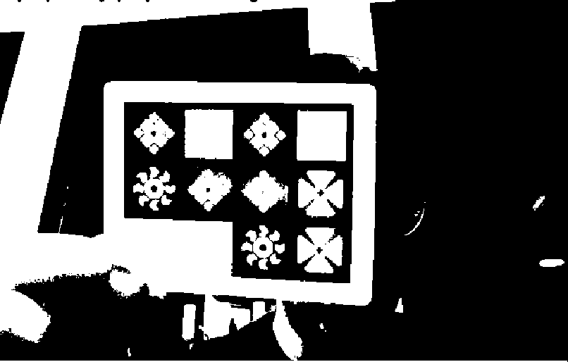
3) Foreground mask

We convert the binary image into a boolean mask (foreground = binary != 0), where True indicates object pixels. This makes logical operations (AND/OR/NOT) easy and fast.

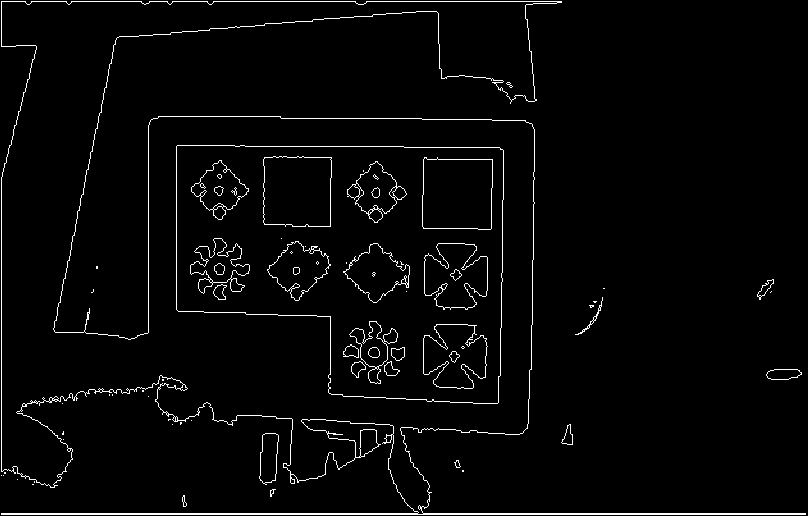
4) Boundary mask

We identify boundary pixels as foreground pixels that are not fully surrounded by foreground in the 4-neighborhood. This produces a thin “outline” that is ideal for contour tracing.

Pseudocode

1
2
3
4
5
6
7
8
9
10
11
12
13
14
15
16
17
18
19
20
21
22
23
24
25
26
27
28
29
30
1. img = threshold(image) 
2. find_contours()
 1. foreground = (img != 0) # set black rgb=0 to true so black is background 
 2. boundary_img = foreground AND NOT(interior_4)
   up = move_up(boundary_image, 1_pixel)
   interior_4 = up AND down AND left AND right
   
 3. visited_boundary = zeros_like(boundary_img, false)
    
 4. neighbor_directions = [(0,1),(1,1),(1,0),(1,-1),(0,-1),(-1,-1),(-1,0),(-1,1)]
        
 5. trace_single_contour(start_row, start_col):
     contour = [(start_row,start_col)]
     visited[start] = True
        current = start
        prev_dir_index = 0   # assume we came from "east" initially
        
     for _ in range(max_steps):
      for direction_idx in range(8):
       point_coord = [current_row, current_col] + neighbor_directions[direction_idx]
       if (boundary[point_coord] == 1):
       next_row, next_col = point_coord
      next_row, next_col  = current_row, current_col
      contour_pixels.append([current_row, current_col])
     return contour_pixels
   1. for each pixel (row,col) in boundary_img:
        if pixel == True and visited[row,col] == False:
            contours.append(trace_single_contour(row,col))

   h) unpad coordinates and return contours

• OpenCV can return different starting points
• OpenCV uses a specific Suzuki-Abe algorithm, can include holes/hierarchy

Step 3 Detect the checkerboard (find the board/card region) TODO

1. If the contour area is too small, skip

2. Compute minAreaRect(contour) to get the best-fit rotated rectangle

3. If the rectangle is too small, skip

4. Track the contour whose rectangle encloses the largest valid area

5. Use cv2.boxPoints(rect) to obtain the 4 corner points (box)

Step 4 Draw the detected board boundary TODO

1
2
3
- Visualize the detected rectangle on the live feed:
    
    `cv2.polylines(overlay, [box.astype(np.int32)], True, (0, 255, 0), 2)`

Step 5 Perspective-warp the board TODO

1
2
3
- Warp the detected quadrilateral into a fixed-size top-down view:
    
    `warped = warp_card(frame, box)`

Step 6 Detect the grid boundaries inside the warped view TODO

1
2
3
- Use the blue grid lines to locate the 3×4 boundaries:
    
    `grid = find_grid_boundaries_from_blue(warped, debug=debug)`

Step 7 Classify each checker cell color TODO

1
2
3
4
5
6
7
8
9
10
11
12
13
14
15
- If grid boundaries were found:
    
    1. Loop over each row and column
        
    2. Extract a central patch (avoid borders/gridlines):
        
        `patch = warped_inner[y0i:y1i, x0i:x1i]`
        
    3. Classify the patch color:
        
        `lbl, conf = classify_cell(patch)`
        
    4. Smooth results over time using a per-cell history:
        
        `hist[r][c].append(lbl) labels[r][c] = mode_label(hist[r][c])`

• Previous
  Robotics - ROS1 Message Processing
• Next
  Robotics Fundamentals - Rotations