Deep Learning - Transformer Series 2 Vanilla Attention Mechanism

Attention Intuition

Imagine we are sitting in a room. We have a red cup of coffee, and a notebook in front of us. When we first sit down, the red cup stands out. So it attracts our attention “involuntarily” to notice the red cup first.

After drinking the coffee, we tell ourselves that “we need to focus on the notebook now”. So we voluntarily and consciously pull our attention to the notebook. Because we are consciously doing it, the attention strength is stronger.

Query-Key-Value (QKV)

When objects enter a machine eye, in our head, they will have a key (a short code), a value (e.g., their pixel values). Based on the machine brain’s “voluntary attention”, the brain will issue a query “what should I see if I want to work?”. They query will be run through all objects’ keys, and based on their similarity (or relavance), each object’s value get assigned to a relavance score, then gets added up, and outputted as the combined “attention”.

More formally, the combined attention is

where the attention weight $\alpha_i$ for the ith key value pair is:

Now, let’s talk about how to calculate the attention score a(q, k_i). There are two types: additive attention, and scaled dot-product attention.

TODO: Intro to key, value

If you come into a library, you know your research question as query. You try to find the shelf number and shelf position of your book, that’s your key. The content of the book you retrieve based on the key is called value. E.g., if your query is “history of the first emperor of Ming Dynasty China”, you then have access to the names of all books in the library (keys), e.g., “Those things in MIng Dynasty”, you can find similarity between the key and your query by their cosine similarity, which is also called “attention” (attn = query * key)

Back to transformer, if you try to learn the wording relationship from individual words in “hi how are you” ,you first convert each word into a vector through the embedding layer. Then you feed each word through 3 different matrices for their query (something interesting about this word), key (unique index of the word), value (the content of the word). For word hi, you get the attention of query hi and key hi = 0.8, hi and how are 0.02, hi and are to be 0.01, hi and you to be 0.1. The learned context vector for “hi” becomes 0.8 * value(hi) + 0.02 * value(how) + 0.02 * value(are) + 0.16 * value(you). This context will be fed though the rest of the system, then each matrix will be updated through back-propagation to minimize some loss function

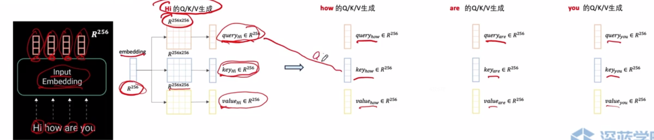
This is self attention, which means words in a sentence will learn from each other (self refers to the sentence itself)

Now, let’s calculate attention:

1
input -> embedding -> 4x256 (each row is an embedding vector for)

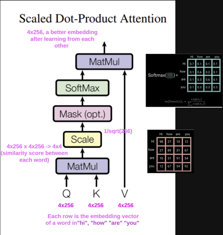Scaling is to normalize the input vectors to the same scale, so they are along similar

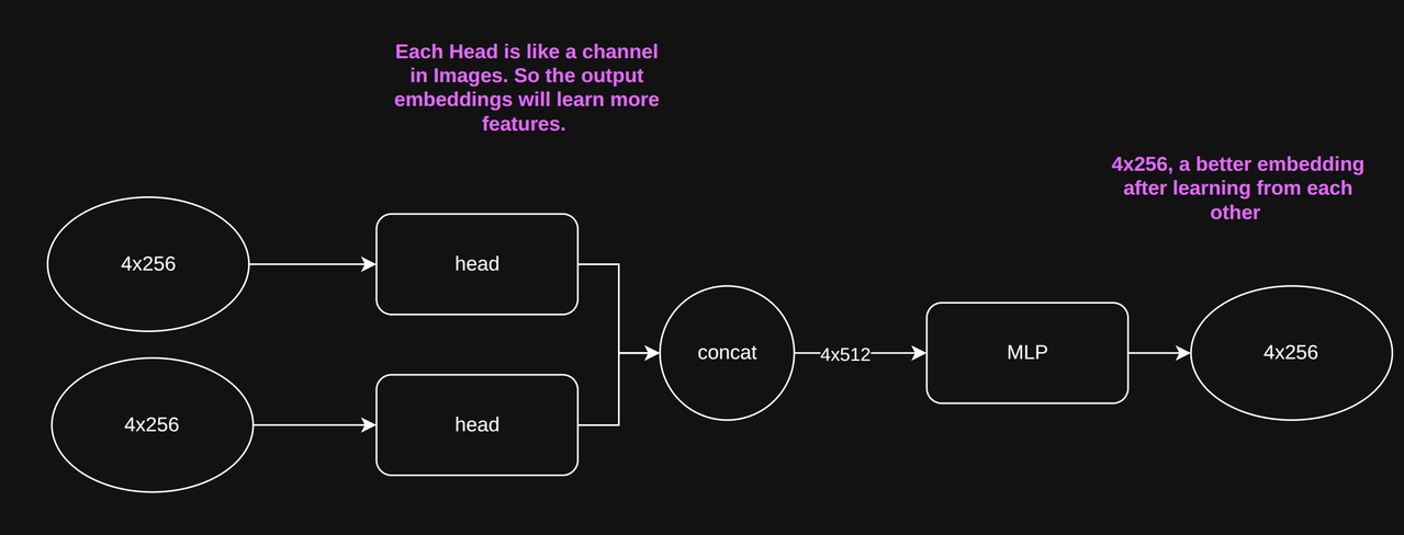
MHSA

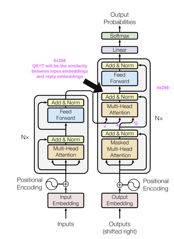
In cross attention,

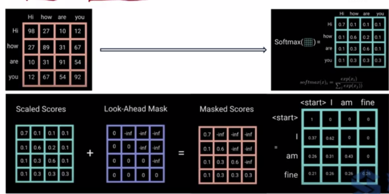
Look-ahead Mask: During text generation (in decoder), the model predicts a token using only previous tokens. E.g., For example, when predicting after ["I", "am"] , the model should not secretly know that the future tokens are: ["fine", "thank", "you", EOS]. By applying a mask, during training, similarities (attention) won’t be calculated for [prev -> future] tokens

Additive (Bahdanau) Attention

When keys and the query have different lengths, we can use the additive attention. Additive attention projects keys and the query into the same length using two linear layers.

The above can be implemented as a single multi-layer perceptron. Below is from the seq2seq tutorial on PyTorch

• key vector k is dk long
• query vector q is dq long
• Say we have h as hidden dimension
• Learnable weight matrices $W_v$ (h, 1), $W_k$ (h, dk), $W_q$ (h, q) score how weighted queries and keys match with each other.

1
2
3
4
5
6
7
8
9
10
11
12
13
14
15
16
17
18
19
20
21
22
23
24
25
26
27
28
29
30
31
32
33
34
35
36
37
38
39
40
41
42
43
44
45
46
47
48
49
50
51
52
53
from torch import nn
import torch

class BahdanauAttention(nn.Module):
    def __init__(self, key_size, query_size, hidden_size, dropout_p):
        super().__init__()
        self.Wk = nn.Linear(key_size, hidden_size, bias=False)
        self.Wq = nn.Linear(query_size, hidden_size, bias=False)
        self.Wv = nn.Linear(hidden_size, 1, bias=False) # a vector
        self.dropout = nn.Dropout(dropout_p)
    def forward(self, queries, keys, values):
        """
        queries: (batch_size, query_num, query_size)
        keys: (batch_size，total_num_key_value_pairs， key_size)
        values: (batch_size，total_num_key_value_pairs， value_size)
        """
        # Project queries and keys onto the same hidden dim
        queries = self.Wq(queries)  # (batch_size, query_num, hidden_size)
        keys = self.Wk(keys)    # (batch_size，total_num_key_value_pairs，hidden_size)
        
        # Broadcasting to add queries and keys together
        queries = queries.unsqueeze(2)  # (batch_size, query_num, 1, hidden_size)
        keys = keys.unsqueeze(1)        # (batch_size, 1, total_num_key_value_pairs, hidden_size)
        features = queries + keys   # (batch_size, query_num, total_num_key_value_pairs, hidden_size)
        features = torch.tanh(features)

        scores = self.Wv(features)  # (batch_size, query_num, total_num_key_value_pairs, 1)
        scores = scores.squeeze(-1) # (batch_size, query_num, total_num_key_value_pairs)
        
        # Use masked_softmax here with a pre-designated length 
        self.attention_weights = nn.functional.softmax(scores)
        
        # torch.bmm is batch-matrix-multiplication
        # (batch_size, query_num, value_size), so we get all queries, weighted
        attention = torch.bmm(self.dropout(self.attention_weights), values)
        return attention

value_size = 2
key_size = 3
query_size = 4
hidden_size = 5
attention = BahdanauAttention(key_size=key_size, query_size=query_size, hidden_size=hidden_size, dropout_p=0.1)

batch_size = 1
query_num = 2
total_num_key_value_pairs = 3

torch.manual_seed(42)
queries = torch.rand((batch_size, query_num, query_size))
keys = torch.rand((batch_size, total_num_key_value_pairs, key_size))
values = torch.rand((batch_size,total_num_key_value_pairs, value_size))

attention(queries, keys, values)

Scaled Dot-Product (Luong) Attention

When keys and queries do have the same length, dot-multiplying them together is faster to give a “relavance” score. Assume Queries is num_queries x hidden_length (d), keys key_pair_num x hidden_length, values key_pair_num x value_length. Below, we denote the length of keys hidden_length as $d_k$

Note that if every pair of elements in keys and queries are independent with [mean=0, var=1], their product $QK^T$ has a zero mean, and a variance d. We normalize this product and choose it to be our attention score a, so its variance is always 1.

The attention mask, a.k.a look-ahead mask M is applied before softmax, after calculating the attention score a (not shown in the illustration). In the attention is all you need paper, the look-ahead mask is applied to make sure future words are not considered in the current step. The “attention is all you need” paper worded this point only with the basic intent, which I found confusing at the first time 😭

1
"We need to prevent leftward information flow in the decoder to preserve the auto-regressive property. We implement this inside of scaled dot-product attention by masking out (setting to −∞) all values in the input of the softmax which correspond to illegal connections"

Then the attention weight is:

This implementation has been tested against the PyTorch MultiHeadAttention Module, given that DotProductAttention is MultiHeadAttention with head=1

All together the code looks like:

1
2
3
4
5
6
7
8
9
10
11
12
13
14
15
16
17
18
19
20
21
22
23
24
25
26
27
28
29
30
31
32
33
34
35
36
37
38
39
class DotProductAttention(torch.nn.Module):
    def forward(
        self,
        q: torch.Tensor,
        k: torch.Tensor,
        v: torch.Tensor,
        attn_mask: torch.Tensor = None,
        key_padding_mask: torch.Tensor = None,
    ):
        """
        Args:
            q (torch.Tensor): [batch_size, query_num, qk_dim] or [batch_size, head_num, query_num, qk_dim]
            k (torch.Tensor): [batch_size, kv_num, qk_dim] or [batch_size, head_num, query_num, qk_dim]
            v (torch.Tensor): [batch_size, kv_num, v_dim] or [batch_size, head_num, query_num, qk_dim]
            attn_mask (torch.Tensor): or look-ahead mask, [query_num, kv_num]. 1 means "mask out"
                Later, they are multiplied by large negative values -1e9. so values can be ignored in softmax.
            key_padding_mask (torch.Tensor): [batch_size, kv_num]. 1 means "mask out"
        Returns:
            attention: [batch_size, query_num, v_dim] or [batch_size, head_num, query_num, qk_dim]
        """
        q_kT_scaled = (q @ k.transpose(-2, -1)) / torch.sqrt(
            torch.tensor(k.shape[-1], dtype=torch.float32)
        )
        if attn_mask is not None:
            q_kT_scaled.masked_fill_(attn_mask.bool(), float("-inf"))
        if key_padding_mask is not None:
            key_padding_mask = key_padding_mask.unsqueeze(1)
            if q_kT_scaled.ndim == 4:
                key_padding_mask = key_padding_mask.unsqueeze(2)
            # [batch_size, query_num, kv_num]
            q_kT_scaled = q_kT_scaled.masked_fill(
                key_padding_mask,
                float("-inf"),
            )
        attention_weight = torch.nn.functional.softmax(q_kT_scaled, dim=-1)
        attention = attention_weight @ v
        # TODO In this implementation, there's a drop out
        # https://ricojia.github.io/2022/03/27/deep-learning-attention-mechanism/#scaled-dot-product-luong-attention
        return attention

Look-Ahead-Mask Omits Paddding For Each Query’s Attention

At timestep t, Padding at in an input sentence start at t. When we train the transformer for a translation task, the decoder gets its last output as its input. So at t, we want to omit <PAD> from then on.

The look ahead mask looks like:

After Applying an look-ahead mask, the attention we get is a weighted sum of all rows in $V$:

• Note that the output attention is [num_queries, value_dimension]. In decoder, only the first self-attention needs this look-ahead mask. The attention’s inputs are outputs from the last timesteps, so num_queries=sentece_length. So effectively, the output attention at each timestep does not consider outputs from a later timestep. Later timesteps are just padding, which will pollute our attention

Visualization of Attention

One great feature about attention is its visibility. Below is an example from the PyTorch NLP page

The input sentence is “il n est pas aussi grand que son pere”.

To interpret:

1. When outputting “he”, most attention was given to “il”, “n”, “est”
2. When outputting “is”, most attention was given to “aussi”, “grand”, “que” (which is interesting because is should be est)
3. When outputting “not”, most attention was given to “aussi”, “pas”, “que”
4. The output “his father” focuses on “son père,” which matches the intended translation.

Bahdanau Encoder-Decoder Structure

Click to expand

In 2014, Bahdanau et al. proposed an encoder-decoder structure **on top of the additive attention**. To illustrate, we have a neural machine translation example (NMT): **translate French input "Jane visite l'Afrique en septembre" to English**. For attention pooling, we talked about scaled dot-product attention pooling and additive attention pooling in the previous sections. - Encoder: we are using a [bi-directional RNN encoder](../2022/2022-03-15-deep-learning-rnn3-lstm.markdown) to generate embeddings of french sentences. Now, our input "Jane visite l'Afrique en septembre" will complete its forward and backward passes. - At each time `t`, the bidirectional RNN encoder outputs **a hidden state** $a^{(t)}$ (which is the key and value at the same time.) - $\alpha^{(t, t')}$: amount of attention output at time `t`, $y^{(t)}$ should put to hidden state at time `t'`, $a^{(t)}$ - Decoder we have **another single-drectional RNN decoder** to generate the word probabilities in the vocab space. - Here, we denote the hidden states as $s^{(t)}$. That's the **query** - Before outputting ``, we assign a weight to several temporal neighbors in the input sequence at each time step.

In this case, we look at 3 neighbors and assign weights to them: $\alpha_1$, $\alpha_2$, $\alpha_3$. So, before outputting "Jane", we look at "Jane", "visite", "l'Afrique" at the same time. Note that this weighted sum of neighbors will enter the RNN cell as the **cell state**. When we read **long** sentences, we have attention for short word segments before finishing the whole sentence. RNN networks's Bleu scores usually dips after a certain length. The attention mechanism, however, has much better performance.

**The process to learn the attention weight $\alpha^{(t, i)}$ is called "alignment"**. "Alignment" is to find the matching patterns between the input and the output. Specifically, alignment is learning the focus to put onto each encoder hidden state. This alignment model is said to **be "soft" so it allows back-propagation** and can be trained with the whole translation model </details> ## References [1] [Bahdanau, D., Cho, K., & Bengio, Y. (2015). Neural machine translation by jointly learning to align and translate. In Proceedings of the 3rd International Conference on Learning Representations (ICLR 2015). https://arxiv.org/abs/1409.0473](https://arxiv.org/pdf/1409.0473) [2] [Xu, K., Ba, J., Kiros, R., Cho, K., Courville, A., Salakhutdinov, R., Zemel, R., and Bengio, Y. 2015. Show, attend and tell: Neural image caption generation with visual attention. In Proceedings of the International Conference on Machine Learning (ICML).](https://arxiv.org/pdf/1502.03044)

• Previous
  Deep Learning - Transformer Series 1 - Embedding Pre-Processing
• Next
  Deep Learning - Transformer Series 3 - Multi-Head and Self Attention