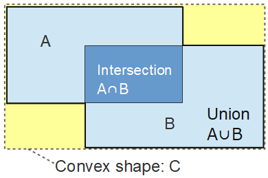
GIoU
Area Under Curve
Area Under Curve = AUC.
True Positives, False Positives, True Negatives, False Negatives
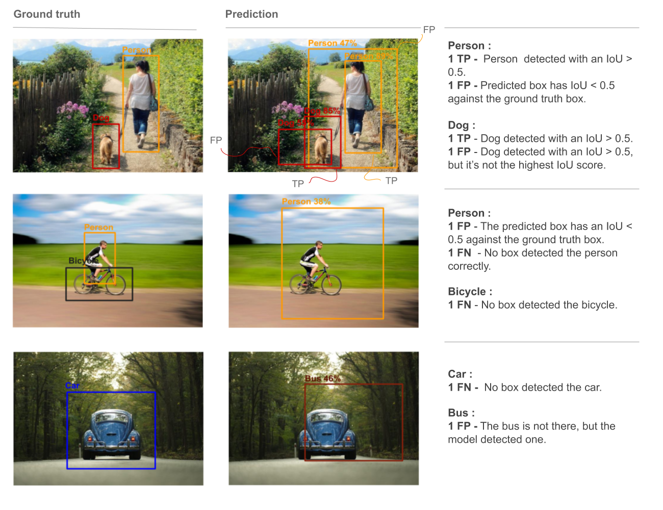
Let’s take an example to illustrate how recall and precision are calculated. Below are images showing objects with ground truth boxes on the left and predictions on the right, and the IoU threshold set to 0.5.
When multiple boxes detect the same object, the box with the highest IoU is considered TP, while the other boxes are FP. If the object is present and the predicted box has an IoU < threshold with the ground truth box, the prediction is considered an FP. More importantly, because no box was detected properly, it also counts as an FN. If the object isn’t present in the image but the model detects one, the prediction counts as an FP. Recall and precision are then computed for each class using the formulas above, by accumulating the counts of TP, FP, and FN.
Average Precision
In this real world example, we have found 7 bounding boxes. We sort them by their confidence
| id | confidence | IoU | Precision | Recall |
|---|---|---|---|---|
| 2 | 0.99 | 0.7 | 0.94 | 0.80 |
| 1 | 0.96 | 0.9 | 0.96 | 0.95 |
| 3 | 0.95 | 0.95 | 1.0 | 0.95 |
| 5 | 0.93 | 0.85 | 1.0 | 0.90 |
| 4 | 0.87 | 0.8 | 1.0 | 0.80 |
| 6 | 0.67 | 0.45 | 0.91 | 0.70 |
Note that the IoU of box 7 is 0. We usually discard boxes with IoU lower than 0.5.. So we discard that one.
Average Precision (AP) is the AUC of the precision-recall curve. In real life, we want a fast way to calculate an approximate of that. Because precision and recall are values in [0, 1], the final AP is also [0, 1]
Mean Average Precision mAP is to take the mean of Average Precion across all classes
\[mAP = \frac{\sum_C AP(c)}{C}\]- AP 50:95: In COCO style object detection evaluation, we take the average of precisions with IoU over 50%. In the case above it will be
mean(0.94 + 0.96 + 1.0 + 1.0 + 1.0)
PASCAL VOC (Visual Object Classes) 11-Point Interpolation, Pre-2010
PASCAL VOC is a common dataset for object detection. Pre-2010, AP is calculated by taking the mean of the highest value in intervals [0.0, 0.1, ... 1.0]. This method is called Interpolated AP
where
\[P_{interpolated}(r) = \max_{\tilde{r} \ge r} P(\tilde{r})\]so when r=0.9, $P_{interpolated}=\max(0.96,1.0,1.0)=1.0$; when r=0.8, ..., we get the same $P_{interpolated}$. The final AP is (1.0 + 1.0 + ...)/11=1.0. The intuition comes from that normally, as recall goes up, precision goes down.
PASCAL VOC (Visual Object Classes) Post-2010
\[\begin{aligned} AP = \sum_r (r_{n+1}-r_{n})P_{interpolated}(r_{n+1}) \\ P_{interpolated}(r_{n+1}) = \max_{\tilde{r} \ge r_{n+1}} P(\tilde{r}) \end{aligned}\]So one difference from PASCAL VOC pre-2010 is we are calculating for every recall level. instead of calculating for the 10 fixed intervals.
Average Recall
| Metric | Meaning |
|---|---|
| AR@1 | Average recall when keeping only the top 1 prediction per image |
| AR@10 | Average recall when keeping top 10 predictions |
| AR@100 | Average recall when keeping top 100 predictions |
| AR_small | Recall for small objects |
| AR_medium | Recall for medium objects |
| AR_large | Recall for large objects |
Average Recall at top 100 means “when allowing maximum 100 predictions per image, how many of the objects are detected”
Confusion Matrix
A confusion matrix shows how often an example whose label is one class (“actual” class) is mislabeled by the algorithm with a different class (“predicted” class). This measures how “confused” a binary classifier is in predictions
| Predicted Positive | Predicted Negative | |
|---|---|---|
| Actual Positive | ||
| Actual Negative |
ROC (Receiver Operating Characteristic Curve)
ROC curve measures the performance of a binary classifier at different decision threshold (TODO what is decision threshold?).
The y axis is True Positive Rate: “what percentage of the positives have you classified” This is the same as “recall” as below
\[\frac{TP}{TP + FN}\]The x axis is False Positive Rate: “what percentage of the negatives have you classified”.
\[\frac{FP}{FP + TN}\]A decision threshold of a binary classifier is the threshold of probability or confidence above which a class can be identified as true. A ROC curve is made when the decision threshold is varied.
- A random classfier would have equal FPR and TPR rates.
Why it’s called ROC: In World War II, the ROC curve was used by the radar operators to detect enemies. Receiver means “radar receiver equipment”, and the curve measures the radar receiver’s ability to distinguish enemies, out of all the enemies, versus false signals like flying objects like birds out of all non-enemy flying objects.
In general, people uses AUC to describe a ROC curve. Pitfalls of ROC include:
- In imbalanced datasets, when positives are rare, even good models might easily have a low TPR, which results in a low ROC value. An example is medical imaging where the positive (disease) could be rare.
- So, negative predicted value should be measured along with ROC
- Precision should be measured along with ROC, see below
The Area-Under-Curve (AUC) of a ROC is always used in plotting the performance of different thresholds of a classifier. The best point on a ROC is (0,1) meaning the True Positive is 1, False Positive is 0. However, people say AUC=1 means a model is good. My question is, what if a model is so good, that its data points clutter around (0,1)? The AUC would be small in that case.
F1 Score
Having a single-value metric makes evaluation intuitive. An F1 score is the “harmonic average” of Precision, and Recall
\[F1 = \frac{2}{\frac{1}{precision} + \frac{1}{recall}}\]F1 score unfortunately is NOT a loss, because it’s NOT differentiable. This is because precion and recall are not differentiable either: each false prediction will contribute either 0 or 1 to the loss, so the loss is calculated discretely, not continuously. To make it continuous, one can use make it a soft F1 Score loss:
\[\begin{aligned} TP = \sum (y_{\text{true}} \cdot y_{\text{pred}}) \\ TN = \sum \left((1 - y_{\text{true}}) \cdot (1 - y_{\text{pred}})\right) \\ FP = \sum \left((1 - y_{\text{true}}) \cdot y_{\text{pred}}\right) \\ FN = \sum \left(y_{\text{true}} \cdot (1 - y_{\text{pred}})\right) \\ \Rightarrow \\ P = \frac{TP}{TP + FP + \epsilon} \\ R = \frac{TP}{TP + FN + \epsilon} \\ F1 = \frac{2 \cdot P \cdot R}{P + R + \epsilon} \end{aligned}\]F1 Score Implementation
1
2
3
4
5
6
7
8
9
10
11
12
13
14
from sklearn.metrics import f1_score
from sklearn.model_selection import train_test_split
from sklearn.datasets import make_classification
from sklearn.ensemble import randomforestclassifier

# generate a synthetic dataset
x, y = make_classification(n_samples=1000, n_features=20, n_classes=2, random_state=42, class_sep=0.8)
x_train, x_test, y_train, y_test = train_test_split(x, y, test_size=0.3, random_state=42)
clf = randomforestclassifier(random_state=42)
clf.fit(x_train, y_train)
y_pred = clf.predict(x_test)
f1 = f1_score(y_test, y_pred)   # array of binary data
# see f1 score: 0.8266666666666667
print(f"f1 score: {f1}")
Satisficing Metric
Satisficing here means “satisfying a certain metric suffices”. It’s a kind of metric that we set a minumum requirement for, but do not care so much afterwards. For example, in a classifier, as long as recall is over 90%, we don’t care about it as much; or in a recommendation system, we set a minimum for speed, but after that we care a lot more on the accuracy.
Cardinality error
Cardinality = number of elements in a set. Cardinality error = number of objects that are mis-classified
Example:
1
2
3
GT objects:        2
model predicts:    4
cardinality error: |4 - 2| = 2
This is usually for logging, not a main optimization loss.
EMA Weights
EMA means Exponential Moving Average of model weights.
Instead of using only the latest weights:
1
current_model_weights
training also maintains smoothed weights:
1
ema_weights = mostly old stable weights + small amount of latest weights
EMA often gives better validation results because it smooths noisy training updates.
So compare:
1
2
val/mAP_50_95
val/ema_mAP_50_95
If EMA is better, use the EMA checkpoint for inference if available.
References
[1] 深入了解平均精度(mAP):通过精确率-召回率曲线评估目标检测性能 [2] mean Average Precision (mAP) — 評估物體偵測模型好壞的指標