Regression Losses
Mean Squared Error (MSE)
\[\text{MSE} = \frac{1}{n}\sum_i (y_i - \hat{y}_i)^2\]- Disadvantages:
- Sensitive to outliers because errors are squared.
- Assumes Gaussian errors; not robust in heavy-tailed noise.
Mean Absolute Error (MAE) / L1 Loss
\[\text{MAE} = \frac{1}{n}\sum_i |y_i - \hat{y}_i|\]nn.L1Loss(reduction="mean") in PyTorch computes this. Example:
1
2
3
4
5
import torch
x = torch.tensor([1., 3., 5.])
y = torch.tensor([2., 1., 5.])
torch.abs(x - y)             # tensor([1., 2., 0.])
torch.mean(torch.abs(x - y)) # tensor(1.0)
reduction options:
"mean"(default): average over all elements → scalar.-
"sum": sum over all elements → $\sum_ix_i - y_i $. -
"none": no reduction → elementwise absolute errors, same shape as inputs. - Advantages: less sensitive to outliers than MSE.
- Disadvantages: not differentiable at 0, which can slow convergence near the minimum.
Hinge Loss
\[\text{Hinge} = \frac{1}{n}\sum_i \max\!\bigl(0,\, 1 - y_i\,\hat{y}_i\bigr)\]Most commonly used in SVM training. Labels should be $\pm 1$. Not well suited to probabilistic outputs.
Huber Loss
Combines the best of MSE (smooth near zero) and MAE (robust to large errors):
\[L_\delta(y,\hat{y}) = \begin{cases} \tfrac{1}{2}(y-\hat{y})^2, & |y-\hat{y}| < \delta, \\ \delta\,|y-\hat{y}| - \tfrac{1}{2}\delta^2, & \text{otherwise.} \end{cases}\]- Advantages: continuous and differentiable everywhere; commonly used in SLAM for robustness to outlier observations.
- Requires tuning $\delta$.
Classification Losses
Cross Entropy Loss (Binary)
For binary classification with predicted probability $\hat{y} \in (0,1)$ and true label $y \in {0,1}$:
\[\text{CE} = -\frac{1}{n}\sum_i \bigl[y_i\log\hat{y}_i + (1-y_i)\log(1-\hat{y}_i)\bigr]\]- Advantages: well-calibrated for probabilistic outputs; penalizes confident wrong predictions heavily.
- Note: the loss diverges as $\hat{y} \to 0$ or $\hat{y} \to 1$, so
BCEWithLogitsLoss(which fuses sigmoid + log) is numerically preferred.
Negative Log-Likelihood Loss (NLL)
NLL measures how likely the model assigns high probability to the true class. Requires log-probability inputs and integer class-index targets (not one-hot vectors).
\[\text{NLL} = -\frac{1}{m}\sum_{j=1}^{m} \log p(y_j \mid x_j)\]Always pair with a log-softmax activation for numerical stability.
Example: logits [1.0, 2.0, 0.5], true class index 1.
- Apply log-softmax:
[-1.463, -0.463, -1.963] - Pick the true-class log-probability: $-\log p(y=1) = 0.463$
Sparse Categorical Cross-Entropy
Used in image segmentation when model outputs per-class probabilities (after softmax) but targets are integer labels rather than one-hot vectors. Loss per sample:
\[l = -\log p_{\text{true}}\]Example: 3 pixels with labels [2, 1, 0] and predicted probability rows:
| Pixel | Class 0 | Class 1 | Class 2 | True class | Loss |
|---|---|---|---|---|---|
| 0 | 0.1 | 0.7 | 0.2 | 2 | $-\log 0.2$ |
| 1 | 0.3 | 0.7 | 0.0 | 1 | $-\log 0.7$ |
| 2 | 0.5 | 0.4 | 0.1 | 0 | $-\log 0.5$ |
Total loss is the sum (or mean) of the per-pixel losses.
Multiclass Classification & Image Segmentation Losses
Multiclass classification and image segmentation both suffer from the data imbalance problem: background pixels or negative classes typically dominate (~80% of samples). The losses below address that imbalance.
IoU and Dice Loss
-
IoU Loss = $1 - \text{IoU}$, where $\text{IoU} = \frac{ \text{intersection} }{ \text{union} }$. -
Dice Loss = $1 - \dfrac{2\, \text{intersection} }{ \text{pred} + \text{target} }$
IoU loss is more sensitive when overlap is low; Dice loss is relatively more sensitive at high overlap (due to the factor of 2 in the numerator). This can be verified by differentiating both expressions.
Simple implementation:
1
2
intersect = (pred == labels).sum().item()
dice_loss = 1.0 - 2 * intersect / (pred.numel() + labels.numel())
Dice loss was introduced alongside weighted cross-entropy for highly imbalanced segmentation by Sudre et al. (2017) [1].
Focal Loss
Focal loss addresses class imbalance by down-weighting easy, well-classified examples so the model focuses on hard ones. The modulating factor $(1-p_t)^\gamma$ shrinks the loss for confident correct predictions. $\gamma \ge 0$ is a hyperparameter; $p_t$ is the predicted probability of the true class.
\[\text{FL}(p_t) = (1-p_t)^{\gamma}\,(-\log p_t)\]
The formulation above assumes each sample has a single true label. For multi-label problems, adaptations are needed — this post explains it well.
1
2
3
4
5
6
7
8
9
10
11
12
13
14
15
16
17
18
19
20
21
22
23
import torch
torch.set_printoptions(precision=4, sci_mode=False, linewidth=150)

num_label = 8
logits  = torch.tensor([[-5., -5, 0.1, 0.1, 5, 5, 100, 100]])
targets = torch.tensor([[0, 1, 0, 1, 0, 1, 0, 1]])

def focal_binary_cross_entropy(logits, targets, gamma=1):
    """
    p_t = sigmoid(logit) for positives, 1 - sigmoid(logit) for negatives.
    - True positive/negative (p_t ≈ 1): (1-p_t) ≈ 0  → small loss ✅
    - False positive/negative (p_t ≈ 0): (1-p_t) ≈ 1  → large loss ✅
    torch.clamp prevents log(0) overflow/underflow.
    """
    l = logits.reshape(-1)
    t = targets.reshape(-1)
    p = torch.sigmoid(l)
    p = torch.where(t >= 0.5, p, 1 - p)           # p_t
    logp = -torch.log(torch.clamp(p, 1e-4, 1 - 1e-4))
    loss = logp * (1 - p) ** gamma                  # focal weight
    return num_label * loss.mean()

focal_binary_cross_entropy(logits, targets)
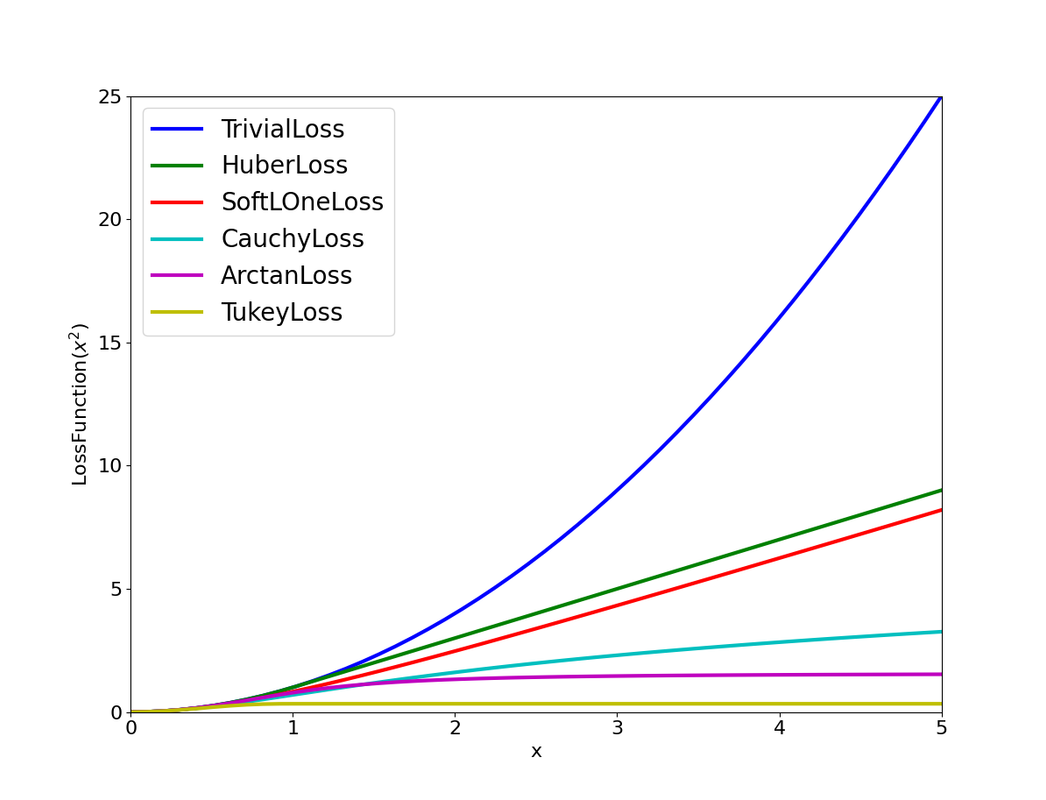
Cauchy Robust Kernel
In typical nonlinear optimization (e.g., SLAM), the squared $L_2$ norm of a residual error $e$ is used as the cost:
\[\begin{gather*} \begin{aligned} & s = e^\top \Omega e \end{aligned} \end{gather*}\]To reduce the influence of outliers, a robust loss function $\rho(s)$ is used in place of the plain quadratic cost. The $\textbf{Cauchy loss}$ is defined as:
\[\begin{gather*} \begin{aligned} & \rho(e) = \delta^2 \ln\left(1 + \frac{e}{\delta^2}\right) \end{aligned} \end{gather*}\]where $\delta$ is a tuning parameter that determines the scale at which residuals begin to be downweighted.
The derivative of the Cauchy loss with respect to $e$ gives the weight applied to the residual during optimization:
\[\begin{gather*} \begin{aligned} & \frac{\partial \rho}{\partial e} = \frac{1}{1 + \frac{e}{\delta^2}} \end{aligned} \end{gather*}\]This expression shows that for large residuals ($s \gg \delta^2$, e.g., a wrong observation edge), the weight decreases, reducing their influence in the optimization process.
Unlike the squared $L_2$ loss, which grows quadratically with $s$, the Cauchy loss grows logarithmically:
- For small $s$, $\rho(s) \approx s$ (behaves like L2).
- For large $s$, $\rho(s)$ grows slowly and the gradient $\frac{\partial \rho}{\partial s}$ asymptotically approaches zero.
References
[1] Sudre, C. H., Li, W., Vercauteren, T., Ourselin, S., & Cardoso, M. J. Generalised Dice overlap as a deep learning loss function for highly unbalanced segmentations. DLMIA/ML-CDS 2017, pp. 240–248.