Robotics - [Motion Planning 1] Overview And A star Variants

The “old school” path planning pipeline is:

1
Path Planning -> Trajectory Optimization

A Star

Setup:

• Maintain a priority_queue to store all nodes to expand
  • The priority queue is initialized with the start state
• Use a heuristic (a guess of future cost to goal from the current state) as a guidance to determine which node to expand next
• Discretize the world into a grid (voxel/pixel).
  • Initialize true cost g(x_s) = 0, other nodes are g(x_n) = inf

Algorithm:

1. If the queue is empty, return false; break
2. Pop the element n with the lowest f(n) = h(n) + g(n) from the queue
   • Mark n as expanded
3. If n is the goal, return
4. For all unexpanded neighbors m of n:
   • If g(m) = infinite,
     • g(m) = g(n) + C_nm
     • Push g(m) to the queue
   • If g(m) > g(n) + C_nm
     • g(m) = g(n) + C_nm

Questions

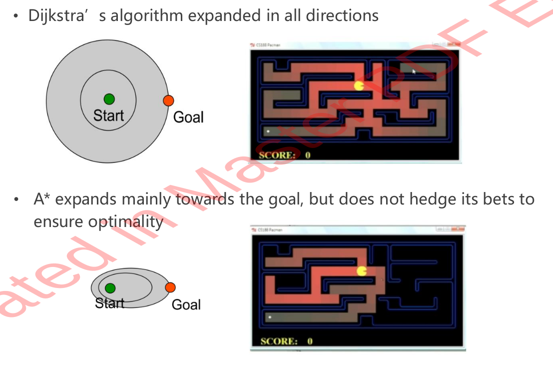
Why must the heuristics be admissible? (h(n) <= actual cost)

When heuristics is admissible, you can find the optimal path:

1. In the extreme case h(n) = 0 (Djikstra’s Algorithm),
   • Nodes on the optimal path are guaranteed to be evaluated.
   • This is because you always evaluate the node with the lowest actual cost.
2. In the regualr admissible case,
   • Because you start from all neighbors at beginning, In the worst case you will evaluate the entire map.
     • Because you will expand “all unexpanded” neighbors
   • In the case where you return when you hit the goal, the queue is not empty:
     • Assume that in the queue, there is another node with smaller true cost T'(n) = g(n') + C_n'goal. Because at the goal, f(goal)=g(goal), we know there are no other nodes that have smaller f(n') = g(n') + h(n'). Meanwhile, admissible heuristics means h(n') < C_n'goal, we can guarantee that no other points in the queue would yield a smaller total cost
   • Unexpanded nodes in the map will have worse f(n'') = g(n'') + h(n'') than the remaining nodes left in the queue, their true cost must be worse than the goal node cost (which is the optimal path cost)

When you have h(n) > actual cost: the search could miss nodes on the optimal path, because there could be a case where:
- When there are nodes left in the queue, their true cost T'(n) = g(n') + C_n'goal might be lower than the goal cost, despite that their f(n') = g(n') + h(n') is larger - Also, the true cost of unexpanded nodes could be lower.

What Does a Good Heuristics Do?

Of course, a good heuristics is in practice what we need to do reduce the search tree. So, L2 norm is always admissible. Manhattan is admissible if you cannot travel in a diagonal manner

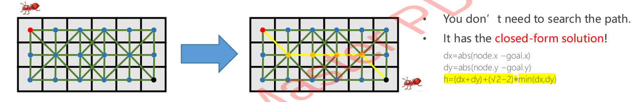
2D, 3D grid world is very structured. One can use a more precise heuristic than L2 norm to reduce the search space (in an entirely empty world):

Is Non-Admissible Heuristics Useless?

Not at all. If we have a weighted $f= g+ \epsilon h$, where a is larger towards the goal, we could have a smaller search space (hence faster), and find a suboptimal route. Weighted A*-> Anytime A*-> ARA*->D*

This is called “$\epsilon$-suboptimality”. It can be orders of magnitude faster than A star

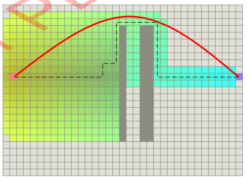
What are the Cons of A Star?

The path could be too close to an obstacle.

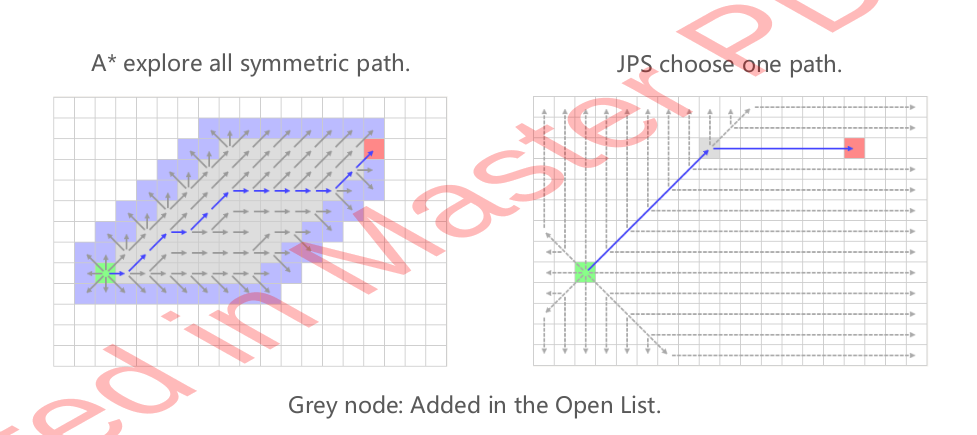
A Star Variant - Jump Point Search (JPS)

JPS is to break symmetry, because vanilla A star will search in the symmetric space:

KinoDynamic Planning

To address the “motion feasible issue” in Vanilla A Star, we can create a graph on velocity, acceleration, and force. This is kinodynamic planning, and the most straight planning is state lattice planning.

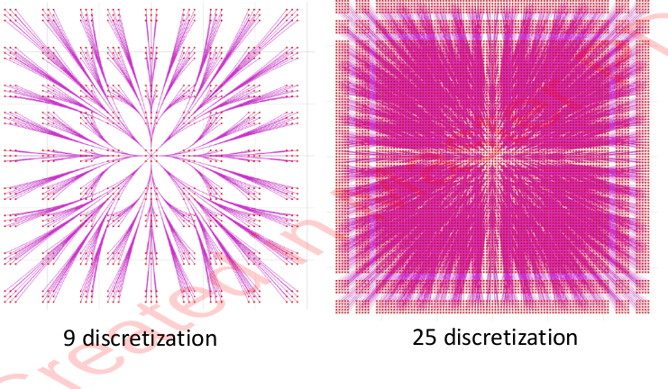
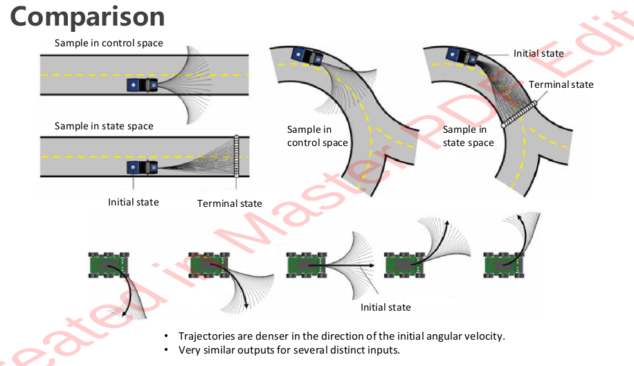
Sampling In Control Space - Low Planning Efficiency

Of course, we live in a discretized world. So one low-planning efficiency method is

1. Sample in control space by: selecting a control vector u
2. Forward simulate the control with numerical integration, for the duration of T:
   • u, T are fixed
3. Assuming acceleration is discretized (that it can change apruptly)
4. State vector is:

Then, we can forward integrate the state using:

If A is “nilpotent”, that is $A^n = 0$, $e^{At}$ has a closed form expression.

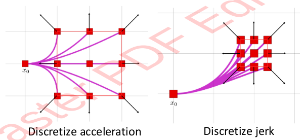
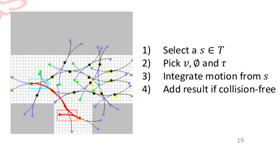
It’s low planning efficiency because it doesn’t provide mission guidance. So we instead sample in State Space:

Sampling In State Space and Reed-Shepp Car Model

1. Given an origin, for 8 neighbors, around the origin, solve for the control required
2. Extend to the outer 24 neighbors

To solve for the control required, one model is the Reeds-Shepp Car Model,

With constraints -1<=v<=1, |k| <= 1/R_min, $R_{min}$ is the minimum arc. So the path is ultimately straight lines and arcs. Reed-Shepp Model allows bi-direction motion (backing up, and forward), and they are non-holonomic feasibility.

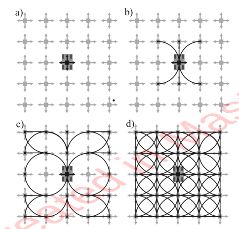
Compared to Control-Space Sampling, State Space sampling yields search-space denser close to its travelling direction

Then, the question becomes: “Design a trajectory that connects x(0) and x(T)”, a.k.a boundary value problem (BVP)

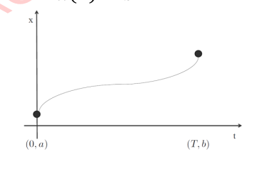
Optimal Boundary Value Problem (OBVP)

1. Example, find a trajectory from t=0 to t=T

• starts at x(0)=a with x′(0)=0, x′′(0)=0,
• ends at x(T)=b with x′(T)=0, x′′(T)=0

TODO

Use Pontryagin’s Minimum Principle to solve for the trajectory, lambda, control input, and the cost. But it’s kind of disgusting.

• Previous
  Computer Vision - Image Downsampling
• Next
  Computer Vision - Random Tree