Metrics
mAP 50 - 95
For each IoU threshold from 0.50 to 0.95, we decide whether each predicted bbox is a true positive by checking whether its IoU with a matched ground-truth box is at least that threshold. Then we sort predictions by confidence, compute the precision-recall curve, calculate AP as the area under that curve, and finally average AP across all IoU thresholds and classes.
- Collect all predictions for that class.
- Sort them from highest confidence to lowest confidence.
- For a fixed IoU threshold, mark each prediction as TP or FP.
- As you move down the confidence-ranked list, compute precision and recall at each step.
- The area under that precision-recall curve is AP.
- Repeat for each IoU threshold.
- Repeat for each class.
- Average across thresholds and classes.
YOLO V1 (Joseph Redmon, Ali Farhadi, 2016)
Before Yolo v1, CNN methods are prevalent, such as R-CNN, Fast R-CNN. These methods would first predict bounding boxes, then classify objects within the bounding boxes. This was slow . YOLO was constructed with 24 convolutional layers and 2 fully connected (FC) layers. This architecture was inspired by GoogLeNet, where convolutional layers learn features while the FC layers output confidence and bounding box coordinates. Therefore, bounding box detection and object classification are implicitly distributed across the network, and the detection speed goes up.

In particular, the bounding box refinement step is ultimately a regression. Its input is a bounding box proposal, e.g., P=(Px,Py,Pw,Ph). The model will output a delta to this prediction: [delta_x, delta_y, delta_w, delta_h].
Additionally, YOLO used:
- Leaky ReLU: like ReLU, but allows a small negative output when the input is negative. This avoids the dying ReLU problem: with normal ReLU, negative inputs become exactly 0, If a neuron keeps receiving negative inputs, its gradient can become zero, and stop learning.
- Dropout: after the first fully connected layer, drop out is turned on such that randomly chosen neurons are turned off amd the network cannot rely too heavily on specific neurons or one specific pathway. Each neuron has to learn features that are useful
- Data Augmentation

YOLO V1 divides the input image into an SxS grid. The center of a cell is responsible for detecting an object that falls into the cell. Every bounding box has a confidence score, so IoU (Intersection over Union) is used to filter out predictions that do not cover most amount of high-confidence cells.
Limitations:
- Each grid cell can only have one class
- Loss function for small bounding boxes is the same for large bounding boxes, which could magnify IoU of the small bboxes.
- Localization Error
YOLO V2 (Joseph Redmon, Ali Farhadi, 2017)
Aka YOLO 9000, YOLO V2 can detect 9000 classes
1
2
3
4
5
6
7
8
9
10
11
12
13
14
15
16
17
18
19
20
21
22
23
24
predictions = model(image)  # many grid-cell / anchor predictions

if sample.type == "detection":
    matched_preds = assign_predictions_to_ground_truth_boxes(predictions, gt_boxes)

    loss_box = box_loss(matched_preds.box, gt_boxes)
    loss_obj = objectness_loss(predictions.obj, gt_objectness)
    loss_cls = wordtree_class_loss(matched_preds.cls, gt_classes)

elif sample.type == "classification":
    selected_pred = choose_prediction_most_responsible_for_class(
        predictions,
        image_level_class
    )

    loss_box = 0.0       # no bbox supervision
    loss_obj = 0.0       # usually ignored
    loss_cls = wordtree_class_loss(
        selected_pred.cls,
        image_level_class
    )

loss = loss_box + loss_obj + loss_cls
loss.backward()
The biggest change is joint training using COCO and Imagenet datasets. COCO has bounding boxes and class labels, with fewer classes. For a detection image, such as COCO:
image + bbox + class label . YOLO 9000 trains L = L_box + L_class + L_confidence. When training with ImageNet data, the model still outputs many bounding boxes. The model only calculates loss for class. Then in back propagation, neurons that do not participate in classification will get close to zero gradient updates.
One note is that We do not pad the output with fake zero bounding boxes because they will teach the robot the wrong things.
Another thing is to infer sub categories probabilities. Say there is a golden retriever image from Imagenet. COCO only has a dog category. YOLO9000 uses a conditional probability
1
2
3
4
5
6
P(Norfolk terrier)
=
P(animal | object)
× P(dog | animal)
× P(terrier | dog)
× P(Norfolk terrier | terrier)
This is done by WordTree. For a COCO output class “dog”, the logit
1
2
3
4
5
6
7
8
9
10
11
12
13
14
15
16
17
18
19
20
21
22
23
24
25
26
27
28
29
30
31
32
33
34
35
36
37
38
39
40
41
42
43
44
45
46
47
48
49
50
51
52
53
54
55
56
57
58
59
60
61
62
63
64
65
66
67
68
69
70
71
72
73
74
75
76
77
78
79
80
81
82
83
84
85
86
class Node:
    def __init__(self, name, parent=None):
        self.name = name
        self.parent = parent
        self.children = []
        self.logit_index = None  # index of this node in the model output

    def add_child(self, child):
        child.parent = self
        self.children.append(child)


# Build tree
object_node = Node("object")

animal = Node("animal")
vehicle = Node("vehicle")
object_node.add_child(animal)
object_node.add_child(vehicle)

dog = Node("dog")
cat = Node("cat")
animal.add_child(dog)
animal.add_child(cat)

terrier = Node("terrier")
shepherd = Node("shepherd")
dog.add_child(terrier)
dog.add_child(shepherd)

norfolk = Node("Norfolk terrier")
yorkshire = Node("Yorkshire terrier")
terrier.add_child(norfolk)
terrier.add_child(yorkshire)

german = Node("German shepherd")
shepherd.add_child(german)

car = Node("car")
boat = Node("boat")
vehicle.add_child(car)
vehicle.add_child(boat)

prediction = {
    "box": box_pred,                  # x, y, w, h
    "objectness": objectness_logit,   # object confidence
    "class_logits": class_logits,     # WordTree logits
}

def conditional_prob(node, class_logits):
    """
    Returns P(node | parent(node)).
    """
    parent = node.parent
    siblings = parent.children

    sibling_indices = [child.logit_index for child in siblings]
    sibling_logits = class_logits[sibling_indices]

    sibling_probs = F.softmax(sibling_logits, dim=0)

    node_position = siblings.index(node)
    return sibling_probs[node_position]

def path_from_root(node):
    path = []
    current = node

    while current.parent is not None:
        path.append(current)
        current = current.parent

    path.reverse()
    return path


def wordtree_probability(target_node, class_logits):
    """
    Computes P(target_node) as product of conditional probabilities.
    """
    prob = torch.tensor(1.0, device=class_logits.device)

    for node in path_from_root(target_node):
        prob = prob * conditional_prob(node, class_logits)

    return prob
YOLOV2 also uses darknet-19 as the backbone. Darknet-19 is a 19-layered CNN.
YOLO V3 Joseph Redmon, Ali Farhadi, 2018)
- multiscale prediction: bounding boxes at 3 different scales, similar to feature pyramid networks. The paper explicitly notes that YOLO had historically struggled with small objects, but multiscale prediction reversed much of that trend.
- Better, and bigger backbone: 53 layered Darknet-53, which suses residual connection but more efficient than ResNet-101 ResNet-152
- Classifier: allows a single box to have multiple labels instead of softmax: each class gets its own sigmoid probability:
class_probs = sigmoid(class_logits), so a box can have probabilities:Person: 0.97 Woman: 0.91 Athlete: 0.74 Dog: 0.01. - Fixed a critical bug in YOLOv2 dataloading, mAP increased by 2% (😂)
On anchor and grid cell:
- scale means the size of the prediction grid.
- An anchor is a pre-chosen bounding box shape that the model uses as a starting guess. YOLO V3 decomposes an image into a 5x5 grid like the above ^. YOLOv3 gives each grid cells a bounding box at a certain scale.
1
2
3
4
# anchors across different grid sizes
"13x13": [(116,90), (156,198), (373,326)],
"26x26": [(30,61), (62,45), (59,119)],
"52x52": [(10,13), (16,30), (33,23)]
Then during training / inference, for each scale, each cell and each anchor,
- the network would predict bounding box position adjustment:
tx, ty,bounding box size adjustment:tw, th - The cell already knows cell position, like
(5,7). anchor height and width , like (156, 198). and stride (how many image pixels one grid step represents). - Finally the model will output the pixel bounding box center
bx, by, bounding box size:bw, bh, class and score
Datasets used was just COCO.
YOLO V4(Alexey Bochkovskiy, Wang, Liao, April 2020)
YOLOV4 is still a one-stage detector. The sparse prediction below could be Faster R-CNN, etc. The biggest improvement is the 3-part architecture:
- head: feature extraction, usually cross-layer CNN to learn features. Here they used CSPDarknet53 , it uses the CSPNet, the Cross-Stage-Partial Network strategy Darknet-53
- neck: Improved spatial pyramid pooling (SPP) and PAN (Path Aggregation Network) to improve granularity of feature extraction from multiple layers of features
- head: YOLOv3’s head to output anchor based?

CSPNet (Cross Stage Partial)
CSPNet paper argues that many CNN stages produce duplicate gradient information. Splitting / merging feature paths would make computation cheaper and gradients diverse. For example, a normal residual stage looks something like:
1
2
3
4
5
def normal_stage(x):
    x = block1(x)
    x = block2(x)
    x = block3(x)
    return x
If x has 256 channels, some gradients might be repeating
1
2
3
256 channels enter
256 channels get processed repeatedly
256 channels exit
Instead, CSP would split the input feature map into two groups. The first group goes through the heavy blocks, the second group skips them,. Finally concatenate these two groups together, like
1
2
3
4
5
6
7
8
9
10
def csp_stage(x):
    x1, x2 = split_channels(x)
    y1 = heavy_blocks(x1)
    y2 = x2
    # Merge both paths
    y = concat(y1, y2)
    # Mix information across channels
    y = transition_conv(y)

    return y
So CSP is basically saying that not every channle needs to go through expensive transformation. Some channels can perserved the original information while the rest are transformed
SPP (Spatial Pyramid Pooling)
YOLO detectors do not usually use the original 2014 SPPNet style SPP. It uses a simpler version:
1
2
3
4
5
feature map
   ├── max pool with small kernel
   ├── max pool with medium kernel
   ├── max pool with large kernel
   └── concatenate all results
This is because convolutional layers have limited receptive field. To augment the context, SPP helps by letting each location gather information from different neighborhood sizes. Maxpooling is a sliding window method with the same stride and padding across different maxpool kernel sizes, so the output feature maps are the same HxW
For example, define maxpool kernels to be: kernel_sizes = [5, 9, 13]. SPP will generate feature maps after maxpooling:
1
2
3
4
x.shape = [B, 512, 13, 13]
p5  = maxpool(x, kernel_size=5,  stride=1, padding=2) # [B, 512, 13, 13]
p9  = maxpool(x, kernel_size=9,  stride=1, padding=4) # [B, 512, 13, 13]
p13 = maxpool(x, kernel_size=13, stride=1, padding=6) # [B, 512, 13, 13]
Then you concatenate them together:
1
2
y = concat([x, p5, p9, p13], dim="channels")
y.shape = [B, 2048, 13, 13]
Usually, people would do a 1x1 convolution to mix / compress the out tensor
An SPP always appear at the end of the backbone or at the start of a neck. Why? Because if placed earlier, SPP would aggregate low-level textures rather than high level textures, and it could be more expensive,. The end of the backbone usually outputs smaller and richer feature maps. SPP is cheaper and could encode more meaningful object level patterns
YOLO V5 (June 2020)
Code Same project as YOLO V8, and YOLO V11
Architecturally, YOLOv5 is closer to the YOLOv3/YOLOv4 generation than to YOLOv8: it uses a PyTorch implementation with a CSP-style backbone/neck and anchor-based detection, while YOLOv8 later introduced an anchor-free split Ultralytics head. YOLOv5’s popularity came from its practical tooling: PyTorch implementation, clean training pipeline, pretrained model zoo, test-time augmentation, model ensembling, and easy export to deployment formats such as ONNX, CoreML, TensorRT, and TFLite
Training on your own data is an iterative loop: collect and label data, train, deploy, inspect failures/edge cases, add more examples, and retrain.
- Collect images, label objects with bounding boxes
- Organize the dataset into YOLO format, create a dataset YAML file listing train/validation
- Image paths and class names, then run YOLOv5’s
train.pyusing a pretrained checkpoint such asyolov5s.pt - After training, the best model is saved as something like
runs/train/exp/weights/best.pt; you can validate it, run inference on new images, then export that trained checkpoint to a deployment format.
SPPF (Spatial Pyramid Pooling - Fast), An Approximation to SPP
Instead of
1
2
3
p1 = maxpool_5x5(x)
p2 = maxpool_9x9(x)
p3 = maxpool_13x13(x)
SPPF repeatedly apply a 5x5 max pool:
1
2
3
4
5
p1 = maxpool_5x5(x)  # 5x5 receptive field
p2 = maxpool_5x5(p1) # 9x9 receptive field
p3 = maxpool_5x5(p2) # 13x13 receptive field

out = concat([x, p1, p2, p3])
YOLO V6 (Meituan Inc, Sep 2022)
YOLO V6 is a practical real-time object detection systems. It can run on commonly available hardware, such as NVIDIA Tesla T4 GPUs. For the backbone, it uses EfficientRep, a hardware-aware CNN design. Smaller models such as YOLOv6-N and YOLOv6-S use RepBlock, while larger models such as YOLOv6-M and YOLOv6-L use CSPStackRep Block to improve representational capacity. For the neck, YOLOv6 adopts Rep-PAN, which builds on the PAN-style feature aggregation used in earlier YOLO models and strengthens it with re-parameterized blocks. This allows the model to fuse features from different backbone levels more efficiently. For the detection head, YOLOv6 introduces an Efficient Decoupled Head, which separates classification and regression while simplifying the convolutional structure to reduce computational cost.
Hardware-aware CNN
“hardware-aware” mainly means the network is designed around operations that are fast and easy to optimize during inference. E.g., YOLOV6 uses RepBlock, inspired by re-parameterization ideas like RepVGG. During training, the block can have multiple branches, which helps the model learn better. During inference, those branches are mathematically fused into a simple convolutional structure.
RepBlock (Re-parameterized Block)
Convolution is a linear operation, batch normalization y = wx + b is also linear. If we have 3x3, 1x1 and identity convolution,and batch normalization, can we combine all of them together? Yes.
Example:
For identity,
1
Identity_kernel =[[0, 0, 0], [0, 1, 0], [0, 0, 0]]
For K1_fused = [[5]],
1
K1_as_3x3 =[[0, 0, 0], [0, 5, 0], [0, 0, 0]]
Then with kernel=3 convolution,
1
K3 =[[1, 2, 1], [0, 1, 0], [2, 1, 0]]
In total you would have a convolution equivalent to:
1
2
3
4
5
K_final = K3_fused + K1_as_3x3 + Kid_as_3x3
K_final =
[[2, 4, 2],
[0, 7.5, 0],
[4, 2, 0]]
So during training, we keep the three branches separately so we are explicitly keeping the original input, and 1x1. The identity branch is especially important. It gives the block an easy way to preserve the input signal. Early in training, a plain conv might distort features randomly. But with an identity branch, the model has a stable path that passes useful information through, which helps gradients flow and makes optimization easier, similar in spirit to residual connections. This helps to achieve K_final in a more stable way even though one can theoretically just keep 1 3x3 convolution block.
1
2
3
branch A: 3x3 Conv + BN
branch B: 1x1 Conv + BN
branch C: Identity + BN
PAN (Path Aggregation Network)
PAN is usually in a neck, which fuses early high resolution feature maps and later low resolution feature maps
1
2
3
4
5
6
7
8
9
10
11
12
13
14
15
16
17
18
19
20
21
22
23
24
25
26
27
Backbone outputs:

P3: high resolution, fine details      80×80
P4: medium resolution                  40×40
P5: low resolution, strong semantics   20×20


FPN top-down path:

P5 ──upsample──► P4
                 │
                 ▼
              fused P4 ──upsample──► P3
                                      │
                                      ▼
                                   fused P3


PAN bottom-up path:

fused P3 ──downsample──► fused P4
                         │
                         ▼
                      fused P4 ──downsample──► fused P5
                                               │
                                               ▼
                                            final P5
- what is the head arch?
YOLO V7 (Jul 2022, Institute of Information Science, Academia Sinica Taiwan)
YOLOv7 is not a radical reinvention of the YOLO architecture, but rather a set of highly practical, fine-grained improvements designed to make real-time object detection more accurate without sacrificing speed. Its main contribution is the use of trainable Bag-of-Freebies: techniques that improve training and representation learning while keeping inference costs low. These include planned re-parameterized convolutions, coarse-to-fine lead-guided label assignment, and extended compound scaling strategies for detection models. In other words, YOLOv7 improves the balance between accuracy and efficiency not by simply making the model larger, but by making the training process and architecture design smarter.
coarse-to-fine lead-guided label assignment
In YOLOV7, an auxiliary head is attached before the final lead head path is fully completed, usually from an intermediate feature stage. It is meant to provide deep supervision: it gives earlier/shallow layers a stronger learning signal during training. The paper describes the lead head’s predictions plus ground truth as guidance for generating coarse-to-fine hierarchical labels, where coarse labels train the auxiliary head and fine labels train the lead head.
lead guided label assignment is like teacher-student style training strategy inside the detector.
Ltotal=Lleadfine+λLauxcoarse
The lead head, which is responsible for the final prediction, is treated as the more reliable “teacher.” Its predictions are used together with the ground-truth boxes to generate soft labels. However, YOLOv7 does not give the same labels to every branch. The auxiliary head receives coarser, more relaxed labels, meaning more candidate boxes are treated as positives so the earlier layers get a stronger and easier learning signal. The lead head receives finer, stricter labels, focusing only on the best-matching candidates for precise final detection. In practice, this helps the model learn broadly first and refine later: the auxiliary branch improves recall and feature learning, while the lead branch sharpens precision. This is why the method is called coarse-to-fine lead-guided label assignment.

Suppose YOLOv7 has 6 candidate prediction boxes near that object. The lead head predicts the following matching scores, where higher means “this candidate looks like a good match to the ground truth.”
| Candidate | IoU with GT | Class confidence | Combined score |
|---|---|---|---|
| A | 0.82 | 0.90 | 0.74 |
| B | 0.76 | 0.85 | 0.65 |
| C | 0.61 | 0.80 | 0.49 |
| D | 0.48 | 0.75 | 0.36 |
| E | 0.35 | 0.70 | 0.25 |
| F | 0.20 | 0.60 | 0.12 |
A fine label assignment might say:
Only candidates with score above 0.50 are positive.
So the lead head trains on:
|Positive for lead head?|Candidates| |—|—| |Yes|A, B| |No|C, D, E, F| A coarse label assignment might relax the threshold:
Candidates with score above 0.30 are positive.
So the auxiliary head trains on:
| Head | Label style | Positive candidates | Purpose |
|---|---|---|---|
| Auxiliary head | Coarse | A, B, C, D | More recall, easier learning |
| Lead head | Fine | A, B | More precision, final detection quality |
YOLO V8 (Jan 10, 2023, Ultralytics)
In spirit, YOLOv8 follows the same direction as YOLOv5: it emphasizes ease of use, fast deployment, and a strong balance between detection accuracy and inference speed.
Architecturally, YOLOv8 introduces an improved backbone and neck, together with an anchor-free detection head. The anchor-free design removes the need for manually predefined anchor boxes, which simplifies the detection pipeline and can improve flexibility across datasets. Beyond detection, Ultralytics also provides YOLOv8 variants for instance segmentation, classification, pose/keypoint detection, and oriented object detection, making it a broader computer vision framework rather than only a single object detector.
improved backbone and neck
YOLOv8 uses C2f modules instead of the older YOLOv5-style C3 modules. C2f roughly means Cross Stage Partial with two convolutions / faster feature fusion. It lets information flow through several lightweight bottleneck paths, then concatenates features together, so the network can preserve more gradient flow and feature diversity without becoming too expensive.
Decoupled Anchor-free detection heads
Problem: anchors are hand-designed or dataset-tuned. If your dataset has unusual object shapes, like long fish, tiny marine debris, or robot parts, anchor choices may not fit well.
YOLOv8 uses an anchor-free detection head, which means it does not rely on predefined anchor boxes. YOLOv8 instead treats each feature-map location as an implicit reference point in the original image. From this point, the model predicts the geometry of the bounding box, such as the distances to the left, top, right, and bottom edges, along with the object class.
YOLOv8 also uses a decoupled head, where classification and box regression are handled by separate branches. The classification branch predicts what object is present, while the box regression branch predicts where the object is located. This design simplifies the detection pipeline, removes the need for manually tuned anchors, and helps YOLOv8 adapt more flexibly to objects with different shapes and scales.

Training UI is very clean (yet to see if it’s fast)
1
2
3
4
5
6
7
8
9
10
11
12
13
14
15
16
17
18
from ultralytics import YOLO
model = YOLO("yolov8s.pt")

# 2. Fine-tune on your dataset
results = model.train(
	data="data.yaml",
	epochs=100,
	imgsz=640,
	batch=16,
	device=0
)

# 3. Validate
metrics = model.val()

# 4. Run inference with your trained model
trained_model = YOLO("runs/detect/train/weights/best.pt")
results = trained_model.predict("test_image.jpg", save=True)
Source: https://docs.ultralytics.com/models/yolov8, https://www.mdpi.com/2073-431X/15/2/74
| Model | COCO mAP50–95 | CPU ONNX latency | A100 TensorRT latency | Params | FLOPs |
|---|---|---|---|---|---|
| YOLOv8n | 37.3 | 80.4 ms | 0.99 ms | 3.2M | 8.7B |
| YOLOv8s | 44.9 | 128.4 ms | 1.20 ms | 11.2M | 28.6B |
| YOLOv8m | 50.2 | 234.7 ms | 1.83 ms | 25.9M | 78.9B |
| YOLOv8l | 52.9 | 375.2 ms | 2.39 ms | 43.7M | 165.2B |
| YOLOv8x | 53.9 | 479.1 ms | 3.53 ms | 68.2M | 257.8B |

YOLO V9 (Feb 2024, 3 bunch of Taiwanese Folks)
Instead of only improving the backbone, neck, label assignment, or detection head, YOLOV9 focuses on a deeper training problem: information loss inside deep neural networks. As an image passes through many layers of feature extraction and spatial transformation, some original input information is inevitably compressed or discarded. This can make the gradients used for learning less reliable.
PGI
YOLOv9 addresses this with Programmable Gradient Information, or PGI, a training strategy that uses an auxiliary reversible branch to preserve richer input information and generate more useful gradient signals. The key idea is that the main network should not only learn from the final detection loss, but also receive better-guided supervision during backpropagation.
The auxiliary branch is reversible in design, so it is less likely to destroy information while producing auxiliary training signals.

Importantly, this auxiliary branch helps during training and can be removed during inference, so it improves learning without adding extra inference cost.

Green arrows is gradient; purple arrows are auxiliary reversible branch and multi-level auxiliary information connections.
At the end of training:
1
2
3
4
5
L_aux → gradient from auxiliary branch
L_total = L_main + λ L_aux

# So finally,
∂L_total/∂W = ∂L_main/∂W + λ ∂L_aux/∂W
Revblock
A Rev Block, or reversible block, is a neural-network block designed so its input can be recovered from its output. Split the input into two parts:
1
2
3
4
5
6
7
8
9
10
11
12
13
14
15
16
17
18
19
20
21
22
# Input feature x is split into two parts along the channel dimension
# x = [x1, x2]
def rev_block_forward(x):
    x1, x2 = split_channels(x)
    # F and G are normal neural network sub-blocks
    # for example: Conv-BN-Activation-Conv
    y1 = x1 + F(x2)
    y2 = x2 + G(y1)
    y = concat_channels(y1, y2)
    return y

# This is NOT used in PGI, but rather a demonstration that there IS a way to recover x from output y. So the network COULD have an easier time infer that
def rev_block_reverse(y):
    y1, y2 = split_channels(y)
    # Reverse the second equation first:
    # y2 = x2 + G(y1)
    x2 = y2 - G(y1)
    # Then reverse the first equation:
    # y1 = x1 + F(x2)
    x1 = y1 - F(x2)
    x = concat_channels(x1, x2)
    return x
in PGI, a Rev Block is not just “another convolution block.” It is a block in the auxiliary training branch that helps keep information available for gradient computation. PGI main mental model is
1
2
3
4
5
6
7
8
9
10
11
12
13
14
15
16
17
18
# Main branch: used at inference
main_features = main_backbone(image)
main_pred = detection_head(main_features)
L_main = detection_loss(main_pred, targets)

# Auxiliary reversible branch: training only
aux_features = rev_branch_forward(image_or_early_features)
aux_pred = auxiliary_head(aux_features)
L_aux = detection_loss(aux_pred, targets)

# Combined training objective
L_total = L_main + lambda_aux * L_aux
L_total.backward()
optimizer.step()

# During inference:
# use only main_backbone + detection_head
# remove rev_branch + auxiliary_head
GELAN
Alongside PGI, YOLOv9 introduces GELAN, or Generalized Efficient Layer Aggregation Network. GELAN can be understood as a more flexible version of ELAN: it is designed to improve information flow through the network while remaining lightweight and efficient. Its structure is based on gradient path planning, meaning the architecture is built with the backward learning signal in mind, not just the forward prediction path.
Gelan keeps the input because not every feature should be forced through deep computation.
1
2
3
4
5
6
7
8
9
10
11
12
13
14
15
16
17
18
19
20
21
def forward(self, x):
    # 1. Project input channels
    x = self.proj(x)  # Conv2d, usually 1x1

    # 2. Split into two channel groups
    x1, x2 = split_channels(x, num_splits=2)

    # 3. Keep short paths and create deeper paths
    y1 = x1                  # short path
    y2 = x2                  # short path

    y3 = self.path1_blocks(x2)
    y4 = self.path2_blocks(y3)

    # 4. Aggregate features from different depths
    y = concat_channels([y1, y2, y3, y4])

    # 5. Fuse aggregated channels
    out = self.fuse(y)       # Conv2d, usually 1x1

    return out
Note: residual connection is a simpler version of GELAN. Residual connection merges by addition, GELAN/ELAN merges by concatenation then fusion.
1
2
def forward(x):
    return x + Block(x)
Together, PGI and GELAN make YOLOv9 stand out because they shift attention from only “how do we predict better boxes?” to “how do we preserve useful information and provide better gradients while training?”

YOLOv9 通过关注信息流和梯度质量,为目标检测提供了全新的视角。PGI 和 GELAN 的引入使 YOLOv9 有别于其前代产品。这种对深度神经网络中信息处理基础的关注,可以提高性能,并更好地解释目标检测中的学习过程。
YOLO V10 (May 2024)
A major limitation of many earlier YOLO models is Non-Maximum Suppression (NMS) as a post-processing step to remove duplicate predictions. Although effective, NMS adds extra latency and makes deployment less clean because the model is not fully end-to-end.
- NMS can become a latency bottleneck: when the scene is crowded and the number of candidate boxes increases, post-processing time can grow and inference latency becomes less predictable.
- NMS is sensitive to manually chosen hyperparameters, especially the IoU threshold. If the threshold is too aggressive, nearby or overlapping objects may be incorrectly removed; if it is too loose, duplicate boxes may remain.
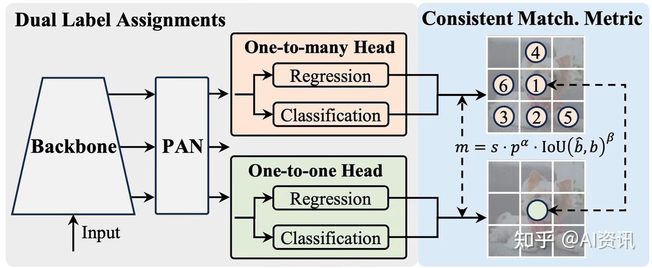
YOLOv10 addresses this with an NMS-free detection strategy based on consistent dual assignments. During training, it uses both one-to-many assignment, which provides rich supervision, and one-to-one assignment, which encourages each object to be matched by a single high-quality prediction. At inference time, YOLOv10 keeps the one-to-one head, allowing it to produce final detections without NMS.
In addition, YOLOv10 introduces a holistic efficiency-accuracy driven design, including lightweight classification heads, spatial-channel decoupled downsampling, and rank-guided block design, to reduce computational cost while preserving detection accuracy. Together, these changes improve the latency-accuracy tradeoff and make YOLOv10 better suited for real-time deployment.
One-to-many head
The one-to-many head is like normal YOLO training.For each ground-truth object, many nearby feature-map locations can be treated as positive examples.
1
2
3
4
5
6
One object:
    fish ground truth
        ↓
    many positive prediction locations
        ↓
    rich training signal
This is good for learning because the model gets many gradients from one object. It helps the backbone and neck learn useful features. But at inference, this creates a problem:
1
same fish → many predicted boxes
So traditional YOLO needs NMS to remove duplicates.
One-to-one head
The one-to-one head is stricter. For each ground-truth object, only one prediction is selected as the positive match.
1
2
3
4
5
6
One object:
    fish ground truth
        ↓
    one best prediction location
        ↓
    one final box
This is what makes NMS-free inference possible. If the model learns to assign only one strong prediction to each object, then you do not need NMS to clean up duplicate boxes.
But one-to-one training alone can be weaker because for one object, only one location gets trained as positive. That means fewer positive gradients.
So YOLOv10 combines both during training, and discard one-to-many head during inference.
1
2
3
4
5
6
7
8
9
10
11
12
13
14
15
16
17
18
19
20
21
22
23
24
25
26
27
28
29
30
31
32
33
def train_step(image, ground_truths):
    # Shared feature extractor
    features = backbone(image)
    features = neck(features)

    # Two heads during training
    preds_many = one_to_many_head(features)
    preds_one  = one_to_one_head(features)

    # Assign labels differently
    targets_many = assign_one_to_many(preds_many, ground_truths)
    targets_one  = assign_one_to_one(preds_one, ground_truths)

    # Compute losses for both heads
    loss_many = detection_loss(preds_many, targets_many)
    loss_one  = detection_loss(preds_one, targets_one)

    # Joint training
    loss = loss_many + loss_one

    loss.backward()
    optimizer.step()

    return loss

def inference(image):
    features = backbone(image)
    features = neck(features)
    # Use only the one-to-one head
    preds = one_to_one_head(features)
    # No NMS needed
    detections = decode_predictions(preds)
    return detections
Matching Score
YOLOv10 uses the idea of a consistent matching metric so the one-to-many and one-to-one heads are not learning contradictory assignments. The metric balances classification confidence and localization quality, so a good match should both classify the object correctly and overlap the ground-truth box well. A simplified pseudo example is
1
2
3
4
5
def matching_score(pred, gt, alpha=1.0, beta=6.0):
    cls_score = pred.class_prob[gt.class_id]
    iou_score = iou(pred.box, gt.box)

    return (cls_score ** alpha) * (iou_score ** beta)
YOLO V11 (Sep 10, 2024, Ultralytics)
YOLO11 made feature extraction more efficient while preserving or slightly improving accuracy. One important change is the introduction of the C3k2 block, an efficient CSP-style module that replaces many of the earlier C2f blocks used in YOLOv8-style designs. Conceptually, C3k2 keeps the benefits of partial feature reuse and gradient flow, but organizes the computation more efficiently so the model can achieve strong performance with fewer parameters and lower computational cost.
YOLO11 also introduces the C2PSA attention block after the SPPF stage, adding position-sensitive/spatial attention to help the model focus on more informative regions of the feature map. Together, C3k2 and C2PSA make YOLO11 feel less like a revolutionary redesign and more like a careful architectural refinement: the model becomes lighter and more efficient while maintaining the real-time detection behavior that makes the YOLO family useful.
C3K2
C3k2 is a lighter CSP/C2f-style feature block. Its job is:
1
2
3
4
5
6
7
8
9
Take input features
↓
split them into shortcut + processed paths
↓
process only part of the channels through small bottleneck blocks
↓
concatenate the paths
↓
fuse everything with a final Conv2d
So conceptually, it is not a totally new idea. The real difference is that a C3k block is a mini CSP module that contains bottlenecks inside it.
1
2
3
4
5
6
7
8
9
10
11
12
13
14
15
class C3k:
	def forward(self, x):
	    a = Conv1x1(x)      # processed path
	    b = Conv1x1(x)      # short CSP path

	    a = bottleneck(a)
	    a = bottleneck(a)

	    return Conv1x1(concat([a, b]))

## Whereas
class Bottleneck:
	# Bottleneck
	def forward(x):
	    return x + Conv(Conv(x))
C2PSA
Same deal with the conventional cross-stage-partial pipeline
1
2
3
4
5
6
7
8
9
10
11
input
  ↓
1×1 Conv projection
  ↓
split channels into two parts
  ├── short path: keep one part mostly unchanged
  └── attention path: send other part through PSA blocks
  ↓
concat short path + attention path
  ↓
1×1 Conv fuse
In principle,
1
2
3
4
5
6
7
8
9
10
11
12
13
14
15
16
17
class C2PSA:
    def forward(self, x):
        # 1. Project channels
        x = Conv2d(x)
        # 2. Split into two feature groups
        x_short, x_attn = split_channels(x, num_splits=2)
        # 3. Keep one branch short
        y_short = x_short
        # 4. Apply position/spatial attention to the other branch
        y_attn = x_attn
        for block in self.psa_blocks:
            y_attn = block(y_attn)
        # 5. Concatenate short branch + attention branch
        y = concat_channels([y_short, y_attn])
        # 6. Fuse channels
        out = self.cv2(y)
        return out
So the real difference is in the PSA block - it uses an attention:
1
2
3
4
5
6
7
8
9
10
class PSABlock:
    def __init__(self, channels):
        self.attn = Attention(channels)
        self.ffn = FeedForward(channels)
    def forward(self, x):
        # Attention branch
        x = x + self.attn(x)
        # Feed-forward / conv branch
        x = x + self.ffn(x)
        return x
YOLO 26 (September 2025, Ultralytics)
YOLO26: An Analysis of NMS-Free End to End Framework for Real-Time Object Detection
AGAIN, Non-Maximum Suppression (NMS) is a PITA. YOLOv10 pioneered an NMS-free direction for YOLO, and YOLO26 further pushes this idea with a native end-to-end design that produces final predictions directly without a separate NMS stage.
1. one-to-one prediction head
During training, the model is “taught” to predict only one most accurate box for each real object, so the model’s output is already the final result, requiring no additional filtering — clean and straightforward. This turns the inference process into a deterministic mapping from input to output, allowing latency to remain stable no matter how complex the scene is.
2. DFL-Free head designed for edge deployment
Recent YOLO versions, such as YOLOv8, commonly use Distribution Focal Loss (DFL) to pursue higher accuracy. DFL treats coordinates as a probability distribution. Although this improves localization accuracy, the Softmax operation it relies on can be very time-consuming on edge devices such as NPUs and DSPs, and it is difficult to quantize. This creates a significant “export gap”: the model may run extremely fast on a GPU, but perform poorly once deployed on edge hardware.
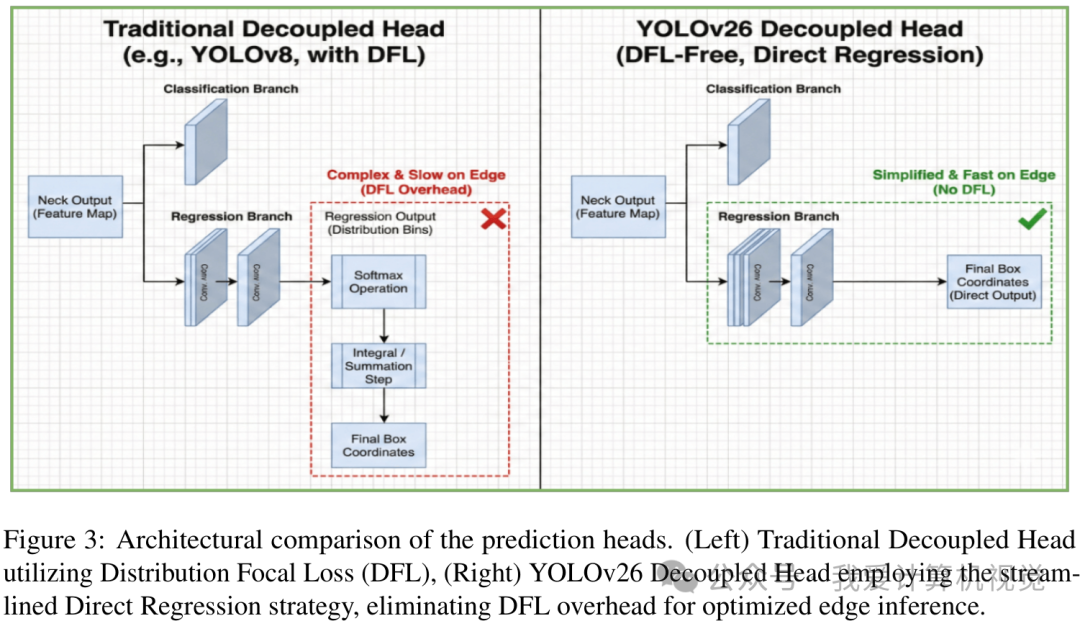
YOLO26 decisively abandons DFL, as shown on the right side of the figure above, and returns to simpler, more hardware-friendly direct coordinate regression. This “rollback” may look like a compromise in accuracy, but in reality, it reflects a strong focus on practical deployment performance.
This raises an important question: after removing two powerful tools, NMS and DFL, how can the model maintain accuracy and still train stably? YOLO26 addresses this with three major training techniques.
1. MuSGD optimizer. see this blogpost
**2. STAL
3. ProgLoss
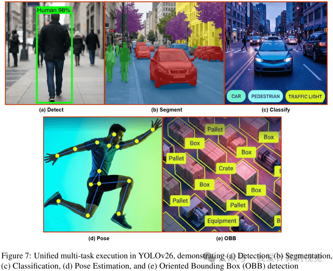
YOLO26’s excellent architecture also makes it a unified multi-task framework. Beyond object detection, it natively supports instance segmentation, pose estimation, oriented bounding box detection, and even open-vocabulary detection through YOLOE-26, demonstrating its significant potential as a next-generation visual foundation model.
What struck me most about YOLO26 is that the field of object detection is shifting away from an arms race focused solely on benchmark metrics and toward deeper thinking about real-world deployment value. Unlike many studies that stack increasingly complex modules to push mAP higher, YOLO26 boldly takes a “less is more” approach. By removing NMS and DFL, it directly addresses the long-standing “Export Gap” problem that has troubled the industry for years.
This shift may be more meaningful than performance numbers alone. After all, the pursuit of accuracy should be grounded in practical usability.
Summary
What’s the mental model of And come up with 5 questions that exposes someone who deeply understand the subject vs someone just understands the fact.
NMS-free inference DFL removal, ProgLoss STAL MuSGD, rather than a DETR-like Transformer redesign.
The use of attention in PSA integration and attention in the later/final stages of the network.So it does have attention-like modules, but these are targeted efficiency/feature-fusion additions, but not a full transformer encoder-decoder object detection framework
Fast 2D / OBB / segmentation front-end
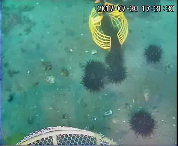
What YOLO does in an underwater Object Detection Dataset
For example, in an underwater robot dataset:
1
small object: distant fish / small toolmedium object: nearby marine animallarge object: diver / robot arm close to camera
A deep feature map has strong semantic understanding but poor spatial detail. A shallow feature map has good spatial detail but weaker semantic understanding.
The neck combines them:
1
shallow feature → where exactly is the object?deep feature    → what is the object?neck fusion     → detect it accurately
This is especially important for small objects because small objects can disappear in deep layers after repeated downsampling.
Underwater Object Detection
Datasets
- URPC 2020 (Underwater Robot Professional Contest, China): 5543 images that showcase four object types: holothurian, echinus, scallop, and starfish